4 Multiple Integration 4.6 Volume Between Surfaces and Triple Integration 5 Vector Analysis

4.7 Triple Integration with Cylindrical and Spherical Coordinates

Just as polar coordinates gave us a new way of describing curves in the plane, in this section we will see how cylindrical and spherical coordinates give us new ways of describing surfaces and regions in space.

Cylindrical Coordinates

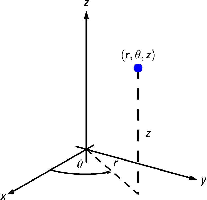
In short, cylindrical coordinates can be thought of as a combination of the polar and rectangular coordinate systems. One can identify a point $(x_{0},y_{0},z_{0})$ , given in rectangular coordinates, with the point $(r_{0},\theta_{0},z_{0})$ , given in cylindrical coordinates, where the $z$ -value in both systems is the same, and the point $(x_{0},y_{0})$ in the $x$ - $y$ plane is identified with the polar point $P(r_{0},\theta_{0})$ ; see Figure 4.49. So that each point in space that does not lie on the $z$ -axis is defined uniquely, we will restrict $r\geq 0$ and $0\leq\theta\leq 2\pi$ .

We use the identity $z=z$ along with the identities found in LABEL:idea:polarconvert to convert between the rectangular coordinate $(x,y,z)$ and the cylindrical coordinate $(r,\theta,z)$ , namely:

Note: Our rectangular to polar conversion formulas used $r^{2}=x^{2}+y^{2}$ , allowing for negative $r$ values. Since we now restrict $r\geq 0$ , we can use $r=\sqrt{x^{2}+y^{2}}$ .

	$\displaystyle\text{From rectangular to cylindrical:}\quad r=\sqrt{x^{2}+y^{2}}% ,\quad\tan\theta=y/x\quad\text{and}\quad z=z;$
	$\displaystyle\text{From cylindrical to rectangular:}\quad x=r\cos\theta\quad y% =r\sin\theta\quad\text{and}\quad z=z.$

These identities, along with conversions related to spherical coordinates, are given later in Key Idea 16.

Watch the video:
Conversion From Rectangular Coordinates from https://youtu.be/w9wCdLuklw8

Example 1 Converting between rectangular and cylindrical coordinates

Convert the rectangular point $(2,-2,1)$ to cylindrical coordinates, and convert the cylindrical point $(4,3\pi/4,5)$ to rectangular.

SolutionFollowing the identities given above (and, later in Key Idea 16), we have $r=\sqrt{2^{2}+(-2)^{2}}=2\sqrt{2}$ . Using $\tan\theta=y/x$ , we find $\theta=\tan^{-1}(-2/2)=-\pi/4$ . As we restrict $\theta$ to being between $0$ and $2\pi$ , we set $\theta=7\pi/4$ . Finally, $z=1$ , giving the cylindrical point $(2\sqrt{2},7\pi/4,1)$ .

In converting the cylindrical point $(4,3\pi/4,5)$ to rectangular, we have $x=4\cos\big{(}3\pi/4\big{)}=-2\sqrt{2}$ , $y=4\sin\big{(}3\pi/4\big{)}=2\sqrt{2}$ and $z=5$ , giving the rectangular point $(-2\sqrt{2},2\sqrt{2},5)$ .

Setting each of $r$ , $\theta$ and $z$ equal to a constant defines a surface in space, as illustrated in the following example.

Figure 4.50: Graphing the canonical surfaces in cylindrical coordinates from Example 2.

Example 2 Canonical surfaces in cylindrical coordinates

Describe the surfaces $r=1$ , $\theta=\pi/3$ and $z=2$ , given in cylindrical coordinates.

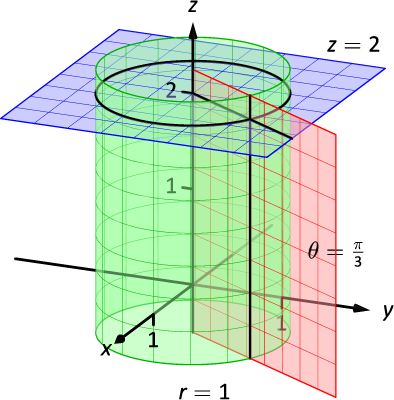
SolutionThe equation $r=1$ describes all points in space that are 1 unit away from the $z$ -axis. This surface is a “tube” or “cylinder” of radius 1, centered on the $z$ -axis, as graphed in Figure 1.8 (which describes the cylinder $x^{2}+y^{2}=1$ in space).

The equation $\theta=\pi/3$ describes the plane formed by extending the line $\theta=\pi/3$ , as given by polar coordinates in the $x$ - $y$ plane, parallel to the $z$ -axis.

The equation $z=2$ describes the plane of all points in space that are 2 units above the $x$ - $y$ plane. This plane is the same as the plane described by $z=2$ in rectangular coordinates.

All three surfaces are graphed in Figure 4.50. Note how their intersection uniquely defines the point $P=(1,\pi/3,2)$ .

Cylindrical coordinates are useful when describing certain domains in space, allowing us to evaluate triple integrals over these domains more easily than if we used rectangular coordinates.

Theorem 44 shows how to evaluate $\iiint_{D}h(x,y,z)\ dV$ using rectangular coordinates. In that evaluation, we use $dV=dz\,dy\,dx$ (or one of the other five orders of integration). Recall how, in this order of integration, the bounds on $y$ are “curve to curve” and the bounds on $x$ are “point to point”: these bounds describe a region $R$ in the $x$ - $y$ plane. We could describe $R$ using polar coordinates as done in Section 4.3. In that section, we saw how we used $dA=r\,dr\,d\theta$ instead of $dA=dy\,dx$ .

Considering the above thoughts, we have $dV=dz\big{(}r\,dr\,d\theta\big{)}=r\,dz\,dr\,d\theta$ . We set bounds on $z$ as “surface to surface” as done in the previous section, and then use “curve to curve” and “point to point” bounds on $r$ and $\theta$ , respectively. Finally, using the identities given above, we change the integrand $h(x,y,z)$ to $h(r,\theta,z)$ .

This process should sound plausible; the following theorem states it is truly a way of evaluating a triple integral.

Theorem 45 Triple Integration in Cylindrical Coordinates

Let $w=h(r,\theta,z)$ be a continuous function on a closed, bounded region $D$ in space, bounded in cylindrical coordinates by $\alpha\leq\theta\leq\beta$ , $g_{1}(\theta)\leq r\leq g_{2}(\theta)$ and $f_{1}(r,\theta)\leq z\leq f_{2}(r,\theta)$ . Then

\iiint_{D}h(r,\theta,z)\ dV=\int_{\alpha}^{\beta}\int_{g_{1}(\theta)}^{g_{2}(% \theta)}\int_{f_{1}(r,\theta)}^{f_{2}(r,\theta)}h(r,\theta,z)r\,dz\,dr\,d\theta.

Figure 4.51: Visualizing the solid used in Example 3.

Example 3 Evaluating a triple integral with cylindrical coordinates

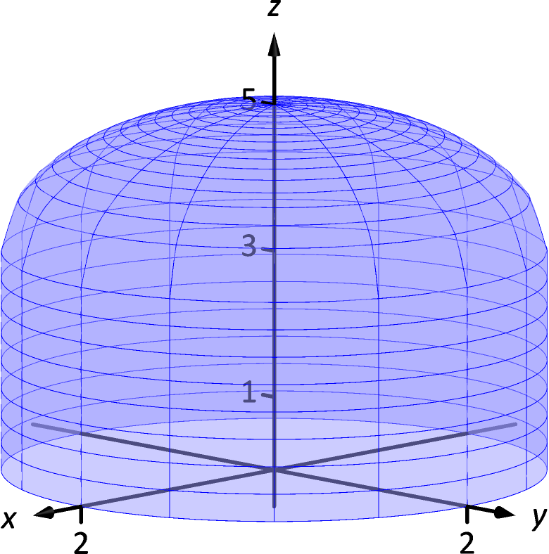
Find the mass of the solid represented by the region in space bounded by $z=0$ , $z=\sqrt{4-x^{2}-y^{2}}+3$ and the cylinder $x^{2}+y^{2}=4$ (as shown in Figure 4.51), with density function $\delta(x,y,z)=x^{2}+y^{2}+z+1$ , using a triple integral in cylindrical coordinates. Distances are measured in centimeters and density is measured in grams/cm ${}^{3}$ .

SolutionWe begin by describing this region of space with cylindrical coordinates. The plane $z=0$ is left unchanged; with the identity $r=\sqrt{x^{2}+y^{2}}$ , we convert the hemisphere of radius 2 to the equation $z=\sqrt{4-r^{2}}$ ; the cylinder $x^{2}+y^{2}=4$ is converted to $r^{2}=4$ , or, more simply, $r=2$ . We also convert the density function: $\delta(r,\theta,z)=r^{2}+z+1$ .

To describe this solid with the bounds of a triple integral, we bound $z$ with $0\leq z\leq\sqrt{4-r^{2}}+3$ ; we bound $r$ with $0\leq r\leq 2$ ; we bound $\theta$ with $0\leq\theta\leq 2\pi$ .

Using Definition 61 and Theorem 45, we have the mass of the solid is

	$\displaystyle M=\iiint_{D}\delta(x,y,z)\ dV$	$\displaystyle=\int_{0}^{2\pi}\int_{0}^{2}\int_{0}^{\sqrt{4-r^{2}}+3}\big{(}r^{% 2}+z+1\big{)}r\,dz\,dr\,d\theta$
		$\displaystyle=\int_{0}^{2\pi}\int_{0}^{2}\big{(}(r^{3}+4r)\sqrt{4-r^{2}}+\frac% {5}{2}r^{3}+\frac{19}{2}r\big{)}\,dr\,d\theta$
		$\displaystyle=\frac{1318\pi}{15}\approx 276.04\text{ gm},$

where we leave the details of the remaining double integral to the reader.

Figure 4.52: Visualizing the solid used in Example 4.

Example 4 Finding the center of mass using cylindrical coordinates

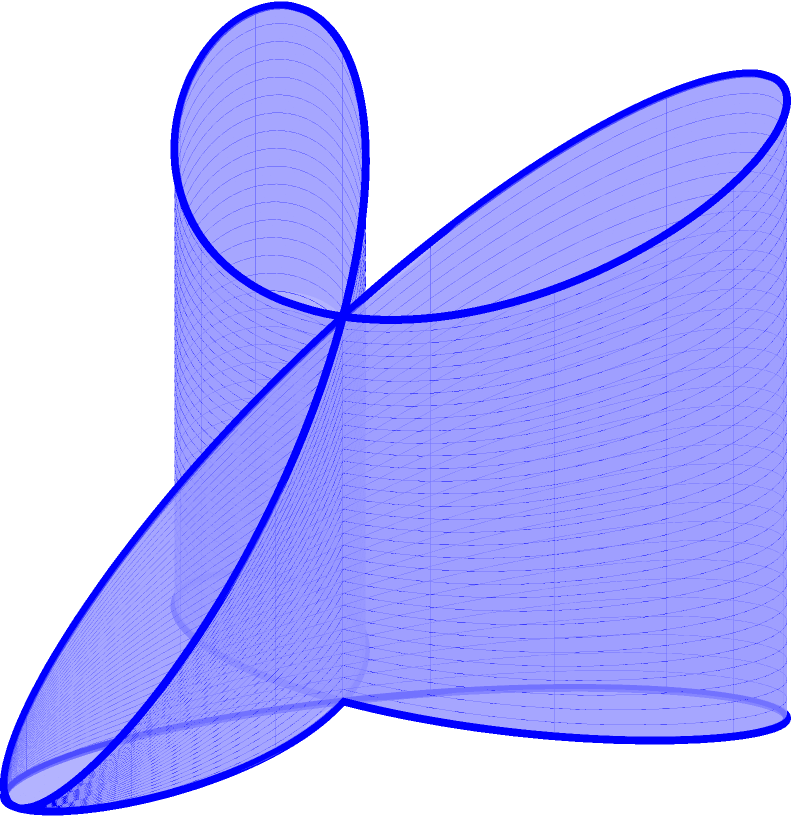
Find the center of mass of the solid with constant density whose base can be described by the polar curve $r=\cos(3\theta)$ and whose top is defined by the plane $z=1-x+0.1y$ , where distances are measured in feet, as seen in Figure 4.52. (The volume of this solid was found in Example 5.)

SolutionWe convert the equation of the plane to use cylindrical coordinates: $z=1-r\cos\theta+0.1r\sin\theta$ . Thus the region is space is bounded by $0\leq z\leq 1-r\cos\theta+0.1r\sin\theta$ , $0\leq r\leq\cos(3\theta)$ , $0\leq\theta\leq\pi$ (recall that the rose curve $r=\cos(3\theta)$ is traced out once on $[0,\pi]$ .

Since density is constant, we set $\delta=1$ and finding the mass is equivalent to finding the volume of the solid. We set up the triple integral to compute this but do not evaluate it; we leave it to the reader to confirm it evaluates to the same result found in Example 5.

M=\iiint_{D}\delta\,dV=\int_{0}^{\pi}\int_{0}^{\cos(3\theta)}\int_{0}^{1-r\cos% \theta+0.1r\sin\theta}r\,dz\,dr\,d\theta\approx 0.785.

From Definition 61 we set up the triple integrals to compute the moments about the three coordinate planes. The computation of each is left to the reader (using technology is recommended):

	$\displaystyle M_{yz}=\iiint_{D}x\,dV$	$\displaystyle=\int_{0}^{\pi}\int_{0}^{\cos(3\theta)}\int_{0}^{1-r\cos\theta+0.% 1r\sin\theta}(r\cos\theta)r\,dz\,dr\,d\theta$
		$\displaystyle=-0.147.$
	$\displaystyle M_{xz}=\iiint_{D}y\,dV$	$\displaystyle=\int_{0}^{\pi}\int_{0}^{\cos(3\theta)}\int_{0}^{1-r\cos\theta+0.% 1r\sin\theta}(r\sin\theta)r\,dz\,dr\,d\theta$
		$\displaystyle=0.015.$
	$\displaystyle M_{xy}=\iiint_{D}z\,dV$	$\displaystyle=\int_{0}^{\pi}\int_{0}^{\cos(3\theta)}\int_{0}^{1-r\cos\theta+0.% 1r\sin\theta}(z)r\,dz\,dr\,d\theta$
		$\displaystyle=0.467.$

The center of mass, in rectangular coordinates, is located at $(-0.147,0.015,0.467)$ , which lies outside the bounds of the solid.

Spherical Coordinates

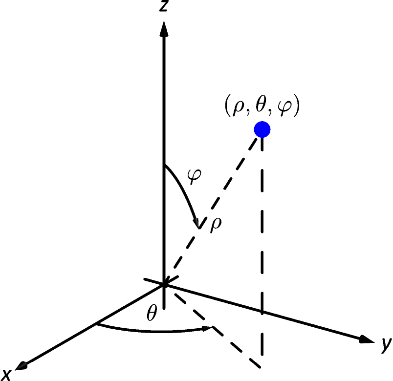
In short, spherical coordinates can be thought of as a “double application” of the polar coordinate system. In spherical coordinates, a point $P$ is identified with $(\rho,\theta,\varphi)$ , where $\rho$ is the distance from the origin to $P$ , $\theta$ is the same angle as would be used to describe $P$ in the cylindrical coordinate system, and $\varphi$ is the angle between the positive $z$ -axis and the ray from the origin to $P$ ; see Figure 4.53. So that each point in space that does not lie on the $z$ -axis is defined uniquely, we will restrict $\rho\geq 0$ , $0\leq\theta\leq 2\pi$ and $0\leq\varphi\leq\pi$ .

Note: The symbol $\rho$ is the Greek letter “rho.” Traditionally it is used in the spherical coordinate system, while $r$ is used in the polar and cylindrical coordinate systems.

The following Key Idea gives conversions to/from our three spatial coordinate systems.

Key Idea 16 Converting Between Rectangular, Cylindrical and Spherical Coordinates

Rectangular and Cylindrical

	$\displaystyle r^{2}=x^{2}+y^{2},\quad\tan\theta=y/x,\quad z=z$
	$\displaystyle x=r\cos\theta,\quad y=r\sin\theta,\quad z=z$

Rectangular and Spherical

	$\displaystyle\rho=\sqrt{x^{2}+y^{2}+z^{2}},\quad\tan\theta=y/x,\quad\cos% \varphi=z/\sqrt{x^{2}+y^{2}+z^{2}}$
	$\displaystyle x=\rho\sin\varphi\cos\theta,\quad y=\rho\sin\varphi\sin\theta,% \quad z=\rho\cos\varphi$

Cylindrical and Spherical

	$\displaystyle\rho=\sqrt{r^{2}+z^{2}},\quad\theta=\theta,\quad\tan\varphi=r/z$
	$\displaystyle r=\rho\sin\varphi,\quad\theta=\theta,\quad z=\rho\cos\varphi$

Note: The role of $\theta$ and $\varphi$ in spherical coordinates differs between mathematicians and physicists. When reading about physics in spherical coordinates, be careful to note how that particular author uses these variables and recognize that these identities will may no longer be valid.

Example 5 Converting between rectangular and spherical coordinates

Convert the rectangular point $(2,-2,1)$ to spherical coordinates, and convert the spherical point $(6,\pi/3,\pi/2)$ to rectangular and cylindrical coordinates.

SolutionThis rectangular point is the same as used in Example 1. Using Key Idea 16, we find $\rho=\sqrt{2^{2}+(-1)^{2}+1^{2}}=3$ . Using the same logic as in Example 1, we find $\theta=7\pi/4$ . Finally, $\cos\varphi=1/3$ , giving $\varphi=\cos^{-1}(1/3)\approx 1.23$ , or about $70.53^{\circ}$ . Thus the spherical coordinates are approximately $(3,7\pi/4,1.23)$ .

Converting the spherical point $(6,\pi/3,\pi/2)$ to rectangular, we have $x=6\sin(\pi/2)\cos(\pi/3)=3$ , $y=6\sin(\pi/2)\sin(\pi/3)=3\sqrt{3}$ and $z=6\cos(\pi/2)=0$ . Thus the rectangular coordinates are $(3,3\sqrt{3},0)$ .

To convert this spherical point to cylindrical, we have $r=6\sin(\pi/2)=6$ , $\theta=\pi/3$ and $z=6\cos(\pi/2)=0$ , giving the cylindrical point $(6,\pi/3,0)$ .

Figure 4.54: Graphing the canonical surfaces in spherical coordinates from Example 6.

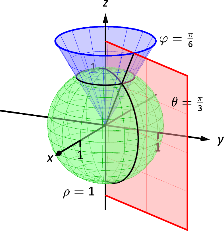
Example 6 Canonical surfaces in spherical coordinates

Describe the surfaces $\rho=1$ , $\theta=\pi/3$ and $\varphi=\pi/6$ , given in spherical coordinates.

SolutionThe equation $\rho=1$ describes all points in space that are 1 unit away from the origin: this is the sphere of radius 1, centered at the origin.

The equation $\theta=\pi/3$ describes the same surface in spherical coordinates as it does in cylindrical coordinates: beginning with the line $\theta=\pi/3$ in the $x$ - $y$ plane as given by polar coordinates, extend the line parallel to the $z$ -axis, forming a plane.

The equation $\varphi=\pi/6$ describes all points $P$ in space where the ray from the origin to $P$ makes an angle of $\pi/6$ with the positive $z$ -axis. This describes a cone, with the positive $z$ -axis its axis of symmetry, with point at the origin.

All three surfaces are graphed in Figure 4.54. Note how their intersection uniquely defines the point $P=(1,\pi/3,\pi/6)$ .

Spherical coordinates are useful when describing certain domains in space, allowing us to evaluate triple integrals over these domains more easily than if we used rectangular coordinates or cylindrical coordinates. The crux of setting up a triple integral in spherical coordinates is appropriately describing the “small amount of volume,” $d V$ , used in the integral.

Considering Figure 4.55, we can make a small “spherical wedge” by varying $\rho$ , $\theta$ and $\varphi$ each a small amount, $\Delta\rho$ , $\Delta\theta$ and $\Delta\varphi$ , respectively. This wedge is approximately a rectangular solid when the change in each coordinate is small, giving a volume of about

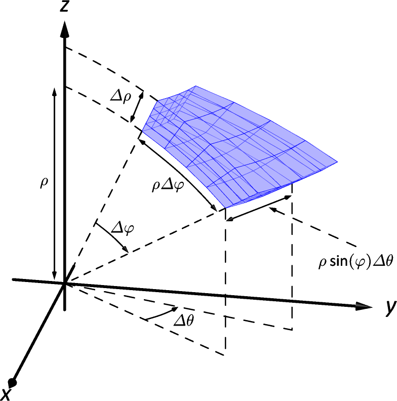
\Delta V\approx\Delta\rho\ \times\ \rho\Delta\varphi\ \times\ \rho\sin(\varphi% )\Delta\theta.

Figure 4.55: Approximating the volume of a standard region in space using spherical coordinates.

Given a region $D$ in space, we can approximate the volume of $D$ with many such wedges. As the size of each of $\Delta\rho$ , $\Delta\theta$ and $\Delta\varphi$ goes to zero, the number of wedges increases to infinity and the volume of $D$ is more accurately approximated, giving

dV=d\rho\ \times\ \rho\ d\varphi\ \times\ \rho\sin(\varphi)d\theta=\rho^{2}% \sin(\varphi)\ d\rho\ d\theta\ d\varphi.

Again, this development of $d V$ should sound reasonable, and the following theorem states it is the appropriate manner by which triple integrals are to be evaluated in spherical coordinates.

Note: It is generally most intuitive to evaluate the triple integral in Theorem 46 by integrating with respect to $\rho$ first; it often does not matter whether we next integrate with respect to $\theta$ or $\varphi$ . Different texts present different standard orders, some preferring $d\varphi\ d\theta$ instead of $d\theta\ d\varphi$ . As the bounds for these variables are usually constants in practice, it generally is a matter of preference.

Theorem 46 Triple Integration in Spherical Coordinates

Let $w=h(\rho,\theta,\varphi)$ be a continuous function on a closed, bounded region $D$ in space, bounded in spherical coordinates by $\alpha_{1}\leq\varphi\leq\alpha_{2}$ , $\beta_{1}\leq\theta\leq\beta_{2}$ and $f_{1}(\theta,\varphi)\leq\rho\leq f_{2}(\theta,\varphi)$ . Then

\iiint_{D}h(\rho,\theta,\varphi)\ dV=\int_{\alpha_{1}}^{\alpha_{2}}\int_{\beta% _{1}}^{\beta_{2}}\int_{f_{1}(\theta,\varphi)}^{f_{2}(\theta,\varphi)}h(\rho,% \theta,\varphi)\rho^{2}\sin(\varphi)\ d\rho\ d\theta\ d\varphi.

Example 7 Establishing the volume of a sphere

Let $D$ be the region in space bounded by the sphere, centered at the origin, of radius $r$ . Use a triple integral in spherical coordinates to find the volume $V$ of $D$ .

SolutionThe sphere of radius $r$ , centered at the origin, has equation $\rho=r$ . To obtain the full sphere, the bounds on $\theta$ and $\varphi$ are $0\leq\theta\leq 2\pi$ and $0\leq\varphi\leq\pi$ . This leads us to:

	$\displaystyle V$	$\displaystyle=\iiint_{D}\ dV$
		$\displaystyle=\int_{0}^{\pi}\int_{0}^{2\pi}\int_{0}^{r}\big{(}\rho^{2}\sin(% \varphi)\big{)}\ d\rho\ d\theta\ d\varphi$
		$\displaystyle=\int_{0}^{\pi}\int_{0}^{2\pi}\left(\frac{1}{3}\rho^{3}\sin(% \varphi)\Big{\|}_{0}^{r}\right)\ d\theta\ d\varphi$
		$\displaystyle=\int_{0}^{\pi}\int_{0}^{2\pi}\left(\frac{1}{3}r^{3}\sin(\varphi)% \right)\ d\theta\ d\varphi$
		$\displaystyle=\int_{0}^{\pi}\left(\frac{2\pi}{3}r^{3}\sin(\varphi)\right)\ d\varphi$
		$\displaystyle=\left.\left(-\frac{2\pi}{3}r^{3}\cos(\varphi)\right)\right\|_{0}^% {\pi}$
		$\displaystyle=\frac{4\pi}{3}r^{3},$

the familiar formula for the volume of a sphere. Note how the integration steps were easy, not using square–roots nor integration steps such as Substitution.

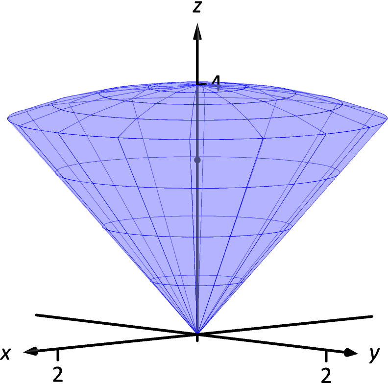
Figure 4.56: Graphing the solid, and its center of mass, from Example 8.

Example 8 Finding the center of mass using spherical coordinates

Find the center of mass of the solid with constant density enclosed above by $\rho=4$ and below by $\varphi=\pi/6$ , as illustrated in Figure 4.56.

SolutionWe will set up the four triple integrals needed to find the center of mass (i.e., to compute $M$ , $M_{yz}$ , $M_{xz}$ and $M_{xy}$ ) and leave it to the reader to evaluate each integral. Because of symmetry, we expect the $x$ - and $y$ - coordinates of the center of mass to be 0.

While the surfaces describing the solid are given in the statement of the problem, to describe the full solid $D$ , we use the following bounds: $0\leq\rho\leq 4$ , $0\leq\theta\leq 2\pi$ and $0\leq\varphi\leq\pi/6$ . Since density $\delta$ is constant, we assume $\delta=1$ .

The mass of the solid:

	$\displaystyle M$	$\displaystyle=\iiint_{D}\ dm=\iiint_{D}\ dV$
		$\displaystyle=\int_{0}^{\pi/6}\int_{0}^{2\pi}\int_{0}^{4}\big{(}\rho^{2}\sin(% \varphi)\big{)}\ d\rho\ d\theta\ d\varphi$
		$\displaystyle=\frac{64}{3}\big{(}2-\sqrt{3}\big{)}\pi\approx 17.958.$

To compute $M_{yz}$ , the integrand is $x$ ; using Key Idea 16, we have $x=\rho\sin\varphi\cos\theta$ . This gives:

	$\displaystyle M_{yz}$	$\displaystyle=\iiint_{D}x\ dm$
		$\displaystyle=\int_{0}^{\pi/6}\int_{0}^{2\pi}\int_{0}^{4}\big{(}(\rho\sin(% \varphi)\cos(\theta))\rho^{2}\sin(\varphi)\big{)}\ d\rho\ d\theta\ d\varphi$
		$\displaystyle=\int_{0}^{\pi/6}\int_{0}^{2\pi}\int_{0}^{4}\big{(}\rho^{3}\sin^{% 2}(\varphi)\cos(\theta)\big{)}\ d\rho\ d\theta\ d\varphi$
		$\displaystyle=0,$

which we expected as we expect $\overline{x}=0$ .

To compute $M_{xz}$ , the integrand is $y$ ; using Key Idea 16, we have $y=\rho\sin\varphi\sin\theta$ . This gives:

	$\displaystyle M_{xz}$	$\displaystyle=\iiint_{D}y\ dm$
		$\displaystyle=\int_{0}^{\pi/6}\int_{0}^{2\pi}\int_{0}^{4}\big{(}(\rho\sin(% \varphi)\sin(\theta))\rho^{2}\sin(\varphi)\big{)}\ d\rho\ d\theta\ d\varphi$
		$\displaystyle=\int_{0}^{\pi/6}\int_{0}^{2\pi}\int_{0}^{4}\big{(}\rho^{3}\sin^{% 2}(\varphi)\sin(\theta)\big{)}\ d\rho\ d\theta\ d\varphi$
		$\displaystyle=0,$

which we also expected as we expect $\overline{y}=0$ .

To compute $M_{xy}$ , the integrand is $z$ ; using Key Idea 16, we have $z=\rho\cos\varphi$ . This gives:

	$\displaystyle M_{xy}$	$\displaystyle=\iiint_{D}z\ dm$
		$\displaystyle=\int_{0}^{\pi/6}\int_{0}^{2\pi}\int_{0}^{4}\big{(}(\rho\cos(% \varphi))\rho^{2}\sin(\varphi)\big{)}\ d\rho\ d\theta\ d\varphi$
		$\displaystyle=\int_{0}^{\pi/6}\int_{0}^{2\pi}\int_{0}^{4}\big{(}\rho^{3}\cos(% \varphi)\sin(\varphi)\big{)}\ d\rho\ d\theta\ d\varphi$
		$\displaystyle=16\pi\approx 50.266.$

Thus the center of mass is $(0,0,M_{xy}/M)\approx(0,0,2.799)$ , as indicated in Figure 4.56.

This section has provided a brief introduction into two new coordinate systems useful for identifying points in space. Each can be used to define a variety of surfaces in space beyond the canonical surfaces graphed as each system was introduced.

However, the usefulness of these coordinate systems does not lie in the variety of surfaces that they can describe nor the regions in space these surfaces may enclose. Rather, cylindrical coordinates are mostly used to describe cylinders and spherical coordinates are mostly used to describe spheres. These shapes are of special interest in the sciences, especially in physics, and computations on/inside these shapes is difficult using rectangular coordinates. For instance, in the study of electricity and magnetism, one often studies the effects of an electrical current passing through a wire; that wire is essentially a cylinder, described well by cylindrical coordinates.

This chapter investigated the natural follow–on to partial derivatives: iterated integration. We learned how to use the bounds of a double integral to describe a region in the plane using both rectangular and polar coordinates, then later expanded to use the bounds of a triple integral to describe a region in space. We used double integrals to find volumes under surfaces, surface area, and the center of mass of lamina; we used triple integrals as an alternate method of finding volumes of space regions and also to find the center of mass of a region in space.

Integration does not stop here. We could continue to iterate our integrals, next investigating “quadruple integrals” whose bounds describe a region in 4–dimensional space (which are very hard to visualize). We can also look back to “regular” integration where we found the area under a curve in the plane. A natural analogue to this is finding the “area under a curve,” where the curve is in space, not in a plane. These are just two of many avenues to explore under the heading of “integration.”

Exercises 4.7

Terms and Concepts

1.

Explain the difference between the roles $r$ , in cylindrical coordinates, and $\rho$ , in spherical coordinates, play in determining the location of a point.
2.

Why are points on the $z$ -axis not determined uniquely when using cylindrical and spherical coordinates?
3.

What surfaces are naturally defined using cylindrical coordinates?
4.

What surfaces are naturally defined using spherical coordinates?

Problems

In Exercises 5–6, points are given in either the rectangular, cylindrical or spherical coordinate systems. Find the coordinates of the points in the other systems.

5.
[-2]
1. (a)
  
  Points in rectangular coordinates:
  
  $(2,2,1)$ and $(-\sqrt{3},1,0)$
2. (b)
  
  Points in cylindrical coordinates:
  
  $(2,\pi/4,2)$ and $(3,3\pi/2,-4)$
3. (c)
  
  Points in spherical coordinates:
  
  $(2,\pi/4,\pi/4)$ and $(1,0,0)$
6.
[-2]
1. (a)
  
  Points in rectangular coordinates:
  
  $(0,1,1)$ and $(-1,0,1)$
2. (b)
  
  Points in cylindrical coordinates:
  
  $(0,\pi,1)$ and $(2,4\pi/3,0)$
3. (c)
  
  Points in spherical coordinates:
  
  $(2,\pi/6,\pi/2)$ and $(3,\pi,\pi)$

In Exercises 7–8, describe the curve, surface or region in space determined by the given bounds.

7.
Bounds in cylindrical coordinates: (a) $r=1$ , $0\leq\theta\leq 2\pi$ , $0\leq z\leq 1$ (b) $1\leq r\leq 2$ , $0\leq\theta\leq\pi$ , $0\leq z\leq 1$

Bounds in spherical coordinates:
1. (c)
  
  $\rho=3$ , $0\leq\theta\leq 2\pi$ , $0\leq\varphi\leq\pi/2$
2. (d)
  
  $2\leq\rho\leq 3$ , $0\leq\theta\leq 2\pi$ , $0\leq\varphi\leq\pi$
8.
Bounds in cylindrical coordinates: (a) $1\leq r\leq 2$ , $\theta=\pi/2$ , $0\leq z\leq 1$ (b) $r=2$ , $0\leq\theta\leq 2\pi$ , $z=5$

Bounds in spherical coordinates:
1. (c)
  
  $0\leq\rho\leq 2$ , $0\leq\theta\leq\pi$ , $\varphi=\pi/4$
2. (d)
  
  $\rho=2$ , $0\leq\theta\leq 2\pi$ , $\varphi=\pi/6$

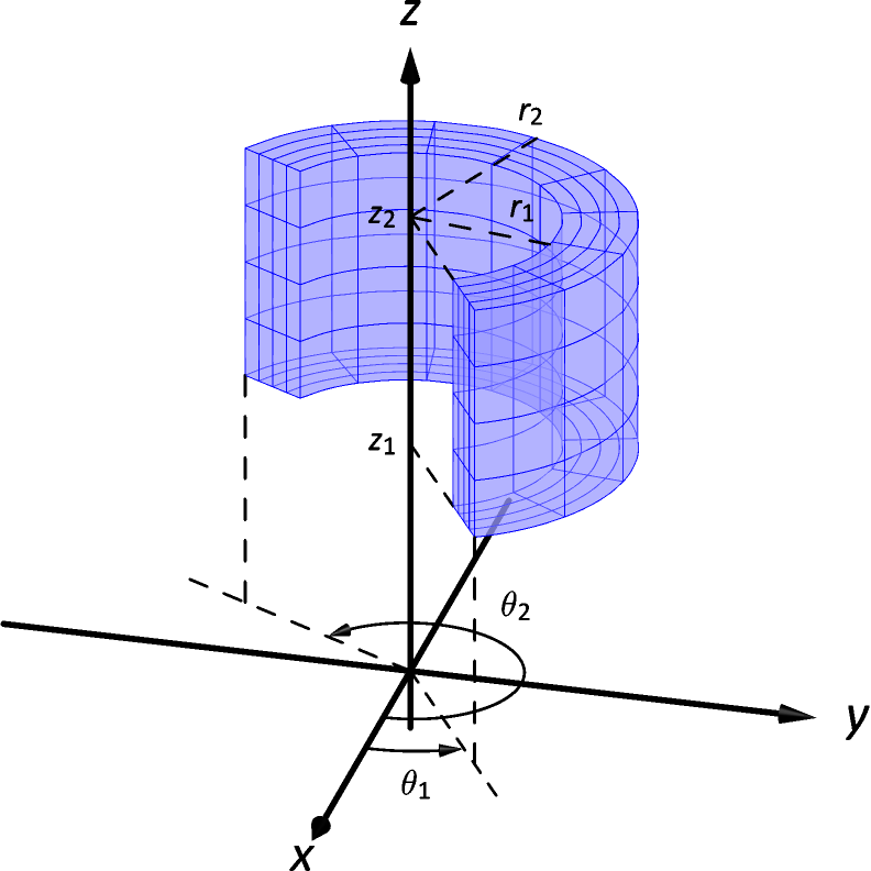
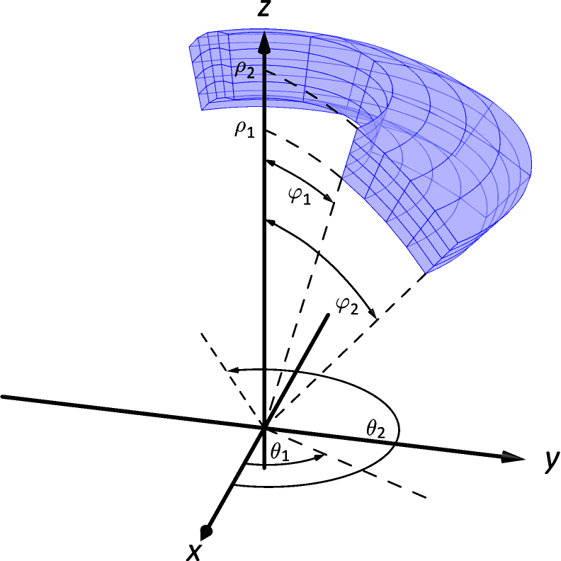
In Exercises 9–10, standard regions in space, as defined by cylindrical and spherical coordinates, are shown. Set up the triple integral that integrates the given function over the graphed region.

9.

Cylindrical coordinates, integrating $h(r,\theta,z)$ :
10.

Cylindrical coordinates, integrating $h(\rho,\theta,\varphi)$ :

In Exercises 11–16, a triple integral in cylindrical coordinates is given. Describe the region in space defined by the bounds of the integral.

11.

$\displaystyle\int_{0}^{\pi/2}\int_{0}^{2}\int_{0}^{2}r\ dz\ dr\ d\theta$
12.

$\displaystyle\int_{0}^{2\pi}\int_{3}^{4}\int_{0}^{5}r\ dz\ dr\ d\theta$
13.

$\displaystyle\int_{0}^{2\pi}\int_{0}^{1}\int_{0}^{1-r}r\ dz\ dr\ d\theta$
14.

$\displaystyle\int_{0}^{\pi}\int_{0}^{1}\int_{0}^{2-r}r\ dz\ dr\ d\theta$
15.

$\displaystyle\int_{0}^{\pi}\int_{0}^{3}\int_{0}^{\sqrt{9-r^{2}}}r\ dz\ dr\ d\theta$
16.

$\displaystyle\int_{0}^{2\pi}\int_{0}^{a}\int_{0}^{\sqrt{a^{2}-r^{2}}+b}r\ dz\ % dr\ d\theta$

In Exercises 17–22, a triple integral in spherical coordinates is given. Describe the region in space defined by the bounds of the integral.

17.

$\displaystyle\int_{0}^{\pi/2}\int_{0}^{\pi}\int_{0}^{1}\rho^{2}\sin(\varphi)\ % d\rho\ d\theta\ d\varphi$
18.

$\displaystyle\int_{0}^{\pi}\int_{0}^{\pi}\int_{1}^{1.1}\rho^{2}\sin(\varphi)\ % d\rho\ d\theta\ d\varphi$
19.

$\displaystyle\int_{0}^{2\pi}\int_{0}^{\pi/4}\int_{0}^{2}\rho^{2}\sin(\varphi)% \ d\rho\ d\theta\ d\varphi$
20.

$\displaystyle\int_{0}^{2\pi}\int_{\pi/6}^{\pi/4}\int_{0}^{2}\rho^{2}\sin(% \varphi)\ d\rho\ d\theta\ d\varphi$
21.

$\displaystyle\int_{0}^{2\pi}\int_{0}^{\pi/6}\int_{0}^{\sec\varphi}\rho^{2}\sin% (\varphi)\ d\rho\ d\theta\ d\varphi$
22.

$\displaystyle\int_{0}^{2\pi}\int_{0}^{\pi/6}\int_{0}^{a\sec\varphi}\rho^{2}% \sin(\varphi)\ d\rho\ d\theta\ d\varphi$

In Exercises 23–26, a solid is described along with its density function. Find the mass of the solid using cylindrical coordinates.

23.

Bounded by the cylinder $x^{2}+y^{2}=4$ and the planes $z=0$ and $z=4$ with density function $\delta(x,y,z)=\sqrt{x^{2}+y^{2}}+1$ .
24.

Bounded by the cylinders $x^{2}+y^{2}=4$ and $x^{2}+y^{2}=9$ , between the planes $z=0$ and $z=10$ with density function $\delta(x,y,z)=z$ .
25.

Bounded by $y\geq 0$ , the cylinder $x^{2}+y^{2}=1$ , and between the planes $z=0$ and $z=4-y$ with density function $\delta(x,y,z)=1$ .
26.

The upper half of the unit ball, bounded between $z=0$ and $z=\sqrt{1-x^{2}-y^{2}}$ , with density function $\delta(x,y,z)=1$ .

In Exercises 27–30, a solid is described along with its density function. Find the center of mass of the solid using cylindrical coordinates. (Note: these are the same solids and density functions as found in Exercises 23 through 26.)

27.

Bounded by the cylinder $x^{2}+y^{2}=4$ and the planes $z=0$ and $z=4$ with density function $\delta(x,y,z)=\sqrt{x^{2}+y^{2}}+1$ .
28.

Bounded by the cylinders $x^{2}+y^{2}=4$ and $x^{2}+y^{2}=9$ , between the planes $z=0$ and $z=10$ with density function $\delta(x,y,z)=z$ .
29.

Bounded by $y\geq 0$ , the cylinder $x^{2}+y^{2}=1$ , and between the planes $z=0$ and $z=4-y$ with density function $\delta(x,y,z)=1$ .
30.

The upper half of the unit ball, bounded between $z=0$ and $z=\sqrt{1-x^{2}-y^{2}}$ , with density function $\delta(x,y,z)=1$ .

In Exercises 31–34, a solid is described along with its density function. Find the mass of the solid using spherical coordinates.

31.

The upper half of the unit ball, bounded between $z=0$ and $z=\sqrt{1-x^{2}-y^{2}}$ , with density function $\delta(x,y,z)=1$ .
32.

The spherical shell bounded between $x^{2}+y^{2}+z^{2}=16$ and $x^{2}+y^{2}+z^{2}=25$ with density function $\delta(x,y,z)=\sqrt{x^{2}+y^{2}+z^{2}}$ .
33.

The conical region bounded above $z=\sqrt{x^{2}+y^{2}}$ and below the sphere $x^{2}+y^{2}+z^{2}=1$ with density function $\delta(x,y,z)=z$ .
34.

The cone bounded above $z=\sqrt{x^{2}+y^{2}}$ and below the plane $z=1$ with density function $\delta(x,y,z)=z$ .

In Exercises 35–38, a solid is described along with its density function. Find the center of mass of the solid using spherical coordinates. (Note: these are the same solids and density functions as found in Exercises 31 through 34.)

35.

The upper half of the unit ball, bounded between $z=0$ and $z=\sqrt{1-x^{2}-y^{2}}$ , with density function $\delta(x,y,z)=1$ .
36.

The spherical shell bounded between $x^{2}+y^{2}+z^{2}=16$ and $x^{2}+y^{2}+z^{2}=25$ with density function $\delta(x,y,z)=\sqrt{x^{2}+y^{2}+z^{2}}$ .
37.

The conical region bounded above $z=\sqrt{x^{2}+y^{2}}$ and below the sphere $x^{2}+y^{2}+z^{2}=1$ with density function $\delta(x,y,z)=z$ .
38.

The cone bounded above $z=\sqrt{x^{2}+y^{2}}$ and below the plane $z=1$ with density function $\delta(x,y,z)=z$ .

In Exercises 39–42, a region is space is described. Set up the triple integrals that find the volume of this region using rectangular, cylindrical and spherical coordinates, then comment on which of the three appears easiest to evaluate.

39.

The region enclosed by the unit sphere, $x^{2}+y^{2}+z^{2}=1$ .
40.

The region enclosed by the cylinder $x^{2}+y^{2}=1$ and planes $z=0$ and $z=1$ .
41.

The region enclosed by the cone $z=\sqrt{x^{2}+y^{2}}$ and plane $z=1$ .
42.

The cube enclosed by the planes $x=0$ , $x=1$ , $y=0$ , $y=1$ , $z=0$ and $z=1$ . (Hint: in spherical, use order of integration $d\rho\ d\varphi\ d\theta$ .)