14 Multiple Integration 14.1 Iterated Integrals and Area 14.3 Double Integration with Polar Coordinates

14.2 Double Integration and Volume

The definite integral of $f$ over $[a,b]$ , $\int_{a}^{b}f(x)\ dx$ , was introduced as “the signed area under the curve.” We approximated the value of this area by first subdividing $[a,b]$ into $n$ subintervals, where the $i^{\text{ th}}$ subinterval has length $\Delta x_{i}$ , and letting $c_{i}$ be any value in the $i^{\text{ th}}$ subinterval. We formed rectangles that approximated part of the region under the curve with width $\Delta x_{i}$ , height $f(c_{i})$ , and hence with area $f(c_{i})\Delta x_{i}$ . Summing all the rectangle’s areas gave an approximation of the definite integral, and Theorem 5.3.2 stated that

\int_{a}^{b}f(x)\ dx=\lim_{\|\Delta x\|\to 0}\sum f(c_{i})\Delta x_{i},

connecting the area under the curve with sums of the areas of rectangles.

We use a similar approach in this section to find volume under a surface.

Let $R$ be a closed, bounded region in the $x$ - $y$ plane and let $z=f(x,y)$ be a continuous function defined on $R$ . We wish to find the signed volume under the surface of $f$ over $R$ . (We use the term “signed volume” to denote that space above the $x$ - $y$ plane, under $f$ , will have a positive volume; space above $f$ and under the $x$ - $y$ plane will have a “negative” volume, similar to the notion of signed area used before.)

^†^†margin: (a)

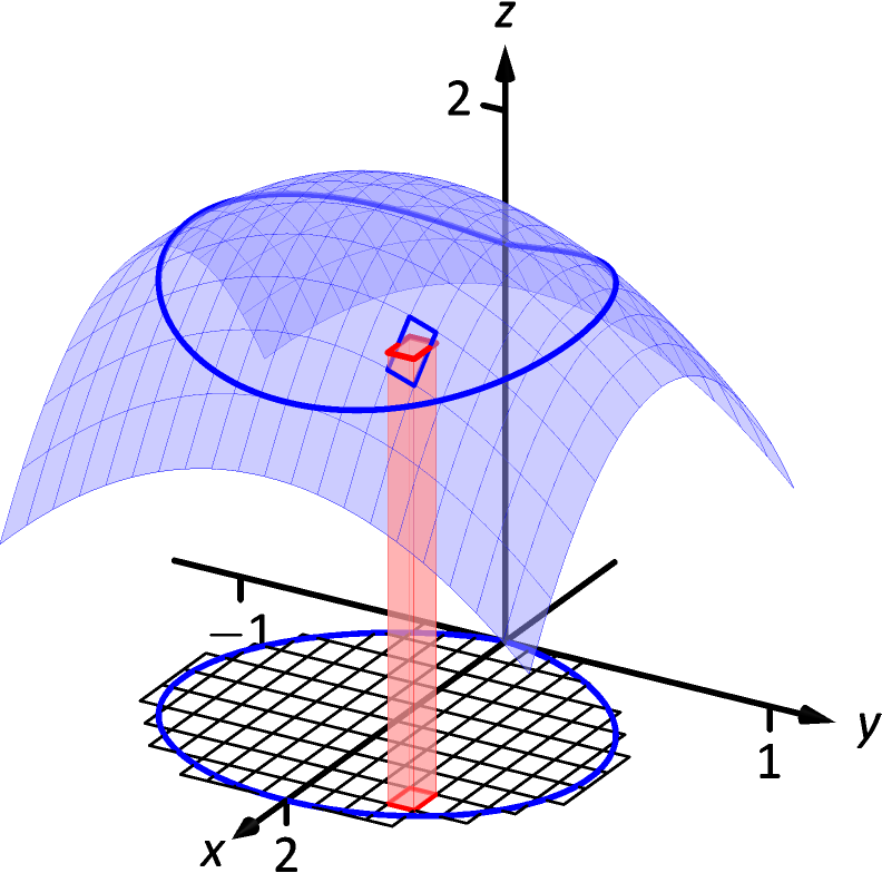(b) Figure 14.2.1: Developing a method for finding signed volume under a surface.

We start by partitioning $R$ into $n$ rectangular subregions as shown in Figure 14.2.1(a). For simplicity’s sake, we let all widths be $\Delta x$ and all heights be $\Delta y$ . Note that the sum of the areas of the rectangles is not equal to the area of $R$ , but rather is a close approximation. Arbitrarily number the rectangles 1 through $n$ , and pick a point $(x_{i},y_{i})$ in the $i^{\text{ th}}$ subregion.

The volume of the rectangular solid whose base is the $i^{\text{ th}}$ subregion and whose height is $f(x_{i},y_{i})$ is $V_{i}=f(x_{i},y_{i})\Delta x\Delta y$ . Such a solid is shown in Figure 14.2.1(b). Note how this rectangular solid only approximates the true volume under the surface; part of the solid is above the surface and part is below.

For each subregion $R_{i}$ used to approximate $R$ , create the rectangular solid with base area $\Delta x\Delta y$ and height $f(x_{i},y_{i})$ . The sum of all rectangular solids is

\displaystyle\sum_{i=1}^{n}f(x_{i},y_{i})\Delta x\Delta y.

This approximates the signed volume under $f$ over $R$ . As we have done before, to get a better approximation we can use more rectangles to approximate the region $R$ .

In general, each rectangle could have a different width $\Delta x_{j}$ and height $\Delta y_{k}$ , giving the $i^{\text{ th}}$ rectangle an area $\Delta A_{i}=\Delta x_{j}\Delta y_{k}$ and the $i^{\text{ th}}$ rectangular solid a volume of $f(x_{i},y_{i})\Delta A_{i}$ . Let $\left\lVert\Delta A\right\rVert$ denote the length of the longest diagonal of all rectangles in the subdivision of $R$ ; $\left\lVert\Delta A\right\rVert\to 0$ means each rectangle’s width and height are both approaching 0. If $f$ is a continuous function, as $\left\lVert\Delta A\right\rVert$ shrinks (and hence $n\to\infty$ ) the summation $\displaystyle\sum_{i=1}^{n}f(x_{i},y_{i})\Delta A_{i}$ approximates the signed volume better and better. This leads to a definition.

^†^†margin: Note: Recall that the integration symbol “

\int

” is an “elongated S,” representing the word “sum.” We interpreted

\int_{a}^{b}f(x)\ dx

as “take the sum of the areas of rectangles over the interval

[a,b]

.” The double integral uses two integration symbols to represent a “double sum.” When adding up the volumes of rectangular solids over a partition of a region

R

, as done in Figure 14.2.1, one could first add up the volumes across each row (one type of sum), then add these totals together (another sum), as in

\sum_{j=1}^{n}\sum_{i=1}^{m}f(x_{i},y_{j})\Delta x_{i}\Delta y_{j}.

One can rewrite this as

\sum_{j=1}^{n}\left(\sum_{i=1}^{m}f(x_{i},y_{j})\Delta x_{i}\right)\Delta y_{j}.

The summation inside the parenthesis indicates the sum of heights

\times

widths, which gives an area; multiplying these areas by the thickness

\Delta y_{j}

gives a volume. The illustration in Figure 14.2.2 relates to this understanding.

Definition 14.2.1 Double Integral, Signed Volume

Let $z=f(x,y)$ be a continuous function defined over a closed region $R$ in the $x$ - $y$ plane. The signed volume $V$ under $f$ over $R$ is denoted by the double integral

V=\iint_{R}f(x,y)\ dA.

Alternate notations for the double integral are

\iint_{R}f(x,y)\ dA=\iint_{R}f(x,y)\ dx\ dy=\iint_{R}f(x,y)\ dy\ dx.

The definition above does not state how to find the signed volume, though the notation offers a hint. We need the next two theorems to evaluate double integrals to find volume.

Theorem 14.2.1 Double Integrals and Signed Volume

Let $z=f(x,y)$ be a continuous function defined over a closed region $R$ in the $x$ - $y$ plane. Then the signed volume $V$ under $f$ over $R$ is

V=\iint_{R}f(x,y)\ dA=\lim_{\left\lVert\Delta A\right\rVert\to 0}\sum_{i=1}^{n% }f(x_{i},y_{i})\Delta A_{i}.

This theorem states that we can find the exact signed volume using a limit of sums. The partition of the region $R$ is not specified, so any partitioning where the diagonal of each rectangle shrinks to 0 results in the same answer.

This does not offer a very satisfying way of computing volume, though. Our experience has shown that evaluating the limits of sums can be tedious. We seek a more direct method.

Recall Theorem 6.2.1 in Section 6.2. This stated that if $A(x)$ gives the cross-sectional area of a solid at $x$ , then $\int_{a}^{b}A(x)\ dx$ gave the volume of that solid over $[a,b]$ .

Consider Figure 14.2.2, where a surface $z=f(x,y)$ is drawn over a region $R$ . Fixing a particular $x$ value, we can consider the area under $f$ over $R$ where $x$ has that fixed value. That area can be found with a definite integral, namely

A(x)=\int_{g_{1}(x)}^{g_{2}(x)}f(x,y)\ dy.

Remember that though the integrand contains $x$ , we are viewing $x$ as fixed. Also note that the bounds of integration are functions of $x$ : the bounds depend on the value of $x$ .

^†^†margin:

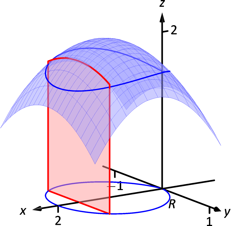Figure 14.2.2: Finding volume under a surface by sweeping out a cross-sectional area.

As $A(x)$ is a cross-sectional area function, we can find the signed volume $V$ under $f$ by integrating it:

V=\int_{a}^{b}A(x)\ dx=\int_{a}^{b}\left(\int_{g_{1}(x)}^{g_{2}(x)}f(x,y)\ dy% \right)dx=\int_{a}^{b}\int_{g_{1}(x)}^{g_{2}(x)}f(x,y)\ dy\ dx.

This gives a concrete method for finding signed volume under a surface. We could do a similar procedure where we started with $y$ fixed, resulting in a iterated integral with the order of integration $dx\ dy$ . The following theorem states that both methods give the same result, which is the value of the double integral. It is such an important theorem it has a name associated with it.

Theorem 14.2.2 Fubini’s Theorem

Let $R$ be a closed, bounded region in the $x$ - $y$ plane and let $z=f(x,y)$ be a continuous function on $R$ .

1.

If $R$ is bounded by $a\leq x\leq b$ and $g_{1}(x)\leq y\leq g_{2}(x)$ , where $g_{1}$ and $g_{2}$ are continuous functions on $[a,b]$ , then

$\iint_{R}f(x,y)\ dA=\int_{a}^{b}\int_{g_{1}(x)}^{g_{2}(x)}f(x,y)\ dy\ dx.$
2.

If $R$ is bounded by $c\leq y\leq d$ and $h_{1}(y)\leq x\leq h_{2}(y)$ , where $h_{1}$ and $h_{2}$ are continuous functions on $[c,d]$ , then

$\iint_{R}f(x,y)\ dA=\int_{c}^{d}\int_{h_{1}(y)}^{h_{2}(y)}f(x,y)\ dx\ dy.$

Note that the bounds of integration follow a “curve to curve, point to point” pattern. In fact, one of the main points of the previous section is developing the skill of describing a region $R$ with the bounds of an iterated integral. Once this skill is developed, we can use double integrals to compute many quantities, not just signed volume under a surface.

Watch the video:
Ex: Evaluate a Double Integral to Determine Volume (Basic) from https://youtu.be/NG2UcXdwzfk

Example 14.2.1 Evaluating a double integral

Let $f(x,y)=xy+e^{y}$ . Find the signed volume under $f$ on the region $R$ , which is the rectangle with corners $(3,1)$ and $(4,2)$ pictured in Figure 14.2.3, using Fubini’s Theorem and both orders of integration.

SolutionWe wish to evaluate $\iint_{R}\big{(}xy+e^{y}\big{)}\ dA$ . As $R$ is a rectangle, the bounds are easily described as $3\leq x\leq 4$ and $1\leq y\leq 2$ .

^†^†margin:

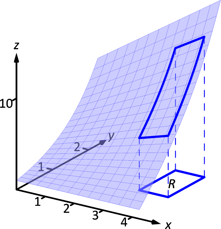Figure 14.2.3: Finding the signed volume under a surface in Example 14.2.1.

Using the order $dy\ dx$ :

	$\displaystyle\iint_{R}\big{(}xy+e^{y}\big{)}\ dA$	$\displaystyle=\int_{3}^{4}\int_{1}^{2}\big{(}xy+e^{y}\big{)}\ dy\ dx$
		$\displaystyle=\int_{3}^{4}\left(\left.\left[\frac{1}{2}xy^{2}+e^{y}\right]% \right\|_{1}^{2}\ \right)dx$
		$\displaystyle=\int_{3}^{4}\left(\frac{3}{2}x+e^{2}-e\right)dx$
		$\displaystyle=\left.\left(\frac{3}{4}x^{2}+\big{(}e^{2}-e\big{)}x\right)\right% \|_{3}^{4}$
		$\displaystyle=\frac{21}{4}+e^{2}-e.$

Now we check the validity of Fubini’s Theorem by using the order $dx\ dy$ :

	$\displaystyle\iint_{R}\big{(}xy+e^{y}\big{)}\ dA$	$\displaystyle=\int_{1}^{2}\int_{3}^{4}\big{(}xy+e^{y}\big{)}\ dx\ dy$
		$\displaystyle=\int_{1}^{2}\left(\left.\left[\frac{1}{2}x^{2}y+xe^{y}\right]% \right\|_{3}^{4}\right)dy$
		$\displaystyle=\int_{1}^{2}\left(\frac{7}{2}y+e^{y}\right)\ dy$
		$\displaystyle=\left.\left(\frac{7}{4}y^{2}+e^{y}\right)\right\|_{1}^{2}$
		$\displaystyle=\frac{21}{4}+e^{2}-e.$

Both orders of integration return the same result, as expected.

Example 14.2.2 Evaluating a double integral

Evaluate $\iint_{R}\big{(}3xy-x^{2}-y^{2}+6\big{)}\ dA$ , where $R$ is the triangle bounded by $x=0$ , $y=0$ and $x/2+y=1$ , as shown in Figure 14.2.4.

SolutionWhile it is not specified which order we are to use, we will evaluate the double integral using both orders to help drive home the point that it does not matter which order we use.

^†^†margin:

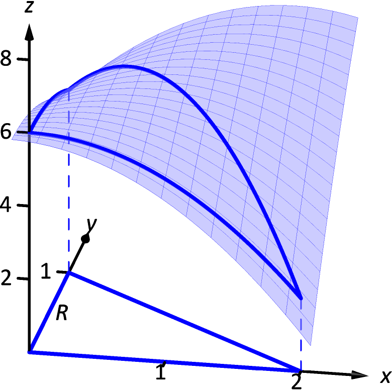Figure 14.2.4: Finding the signed volume under the surface in Example 14.2.2.

Using the order $dy\ dx$ : The bounds on $y$ go from “curve to curve,” i.e., $0\leq y\leq 1-x/2$ , and the bounds on $x$ go from “point to point,” i.e., $0\leq x\leq 2$ .

	$\displaystyle\iint_{R}(3xy-x^{2}-y^{2}+6\big{)}\ dA$	$\displaystyle=\int_{0}^{2}\int_{0}^{-\frac{x}{2}+1}(3xy-x^{2}-y^{2}+6\big{)}\ % dy\ dx$
		$\displaystyle=\int_{0}^{2}\left.\left(\frac{3}{2}xy^{2}-x^{2}y-\frac{1}{3}y^{3% }+6y\right)\right\|_{0}^{-\frac{x}{2}+1}dx$
		$\displaystyle=\int_{0}^{2}\left(\frac{11}{12}x^{3}-\frac{11}{4}x^{2}-x+\frac{1% 7}{3}\right)dx$
		$\displaystyle=\left.\left(\frac{11}{48}x^{4}-\frac{11}{12}x^{3}-\frac{1}{2}x^{% 2}+\frac{17}{3}x\right)\right\|_{0}^{2}$
		$\displaystyle=\frac{17}{3}=5.\overline{6}.$

Now lets consider the order $dx\ dy$ . Here $x$ goes from “curve to curve,” $0\leq x\leq 2-2y$ , and $y$ goes from “point to point,” $0\leq y\leq 1$ :

	$\displaystyle\iint_{R}(3xy-x^{2}-y^{2}+6\big{)}\ dA$	$\displaystyle=\int_{0}^{1}\int_{0}^{2-2y}(3xy-x^{2}-y^{2}+6\big{)}\ dx\ dy$
		$\displaystyle=\int_{0}^{1}\left.\left(\frac{3}{2}x^{2}y-\frac{1}{3}x^{3}-xy^{2% }+6x\right)\right\|_{0}^{2-2y}dy$
		$\displaystyle=\int_{0}^{1}\left(\frac{32}{3}y^{3}-22y^{2}+2y+\frac{28}{3}% \right)dy$
		$\displaystyle=\left.\left(\frac{8}{3}y^{4}-\frac{22}{3}y^{3}+y^{2}+\frac{28}{3% }y\right)\right\|_{0}^{1}$
		$\displaystyle=\frac{17}{3}=5.\overline{6}.$

We obtained the same result using both orders of integration.

Note how in these two examples that the bounds of integration depend only on $R$ ; the bounds of integration have nothing to do with $f(x,y)$ . This is an important concept, so we include it as a Key Idea.

Key Idea 14.2.1 Double Integration Bounds

When evaluating $\iint_{R}f(x,y)\ dA$ using an iterated integral, the bounds of integration depend only on $R$ . The surface $f$ does not determine the bounds of integration.

Before doing another example, we give some properties of double integrals. Each should make sense if we view them in the context of finding signed volume under a surface, over a region.

Theorem 14.2.3 Properties of Double Integrals

Let $f$ and $g$ be continuous functions over a closed, bounded plane region $R$ , and let $c$ be a constant.

1.

$\displaystyle\iint_{R}c\,f(x,y)\ dA=c\iint_{R}f(x,y)\ dA.$
2.

$\displaystyle\iint_{R}\big{(}f(x,y)\pm g(x,y)\big{)}\ dA=\iint_{R}f(x,y)\ dA% \pm\iint_{R}g(x,y)\ dA$
3.

If $f(x,y)\geq 0$ on $R$ , then $\displaystyle\iint_{R}f(x,y)\ dA\geq 0$ .
4.

If $f(x,y)\geq g(x,y)$ on $R$ , then $\displaystyle\iint_{R}f(x,y)\ dA\geq\iint_{R}g(x,y)\ dA$ .
5.

Let $R$ be the union of two nonoverlapping regions, $R=R_{1}\bigcup R_{2}$ (see Figure 14.2.5). Then

$\iint_{R}f(x,y)\ dA=\iint_{R_{1}}f(x,y)\ dA+\iint_{R_{2}}f(x,y)\ dA.$

^†^†margin: Figure 14.2.5:

R

is the union of two nonoverlapping regions,

R_{1}

and

R_{2}

Example 14.2.3 Evaluating a double integral

Let $f(x,y)=\sin x\cos y$ and $R$ be the triangle with vertices $(-1,0)$ , $(1,0)$ and $(0,1)$ (see Figure 14.2.6). Evaluate the double integral $\iint_{R}f(x,y)\ dA$ . ^†^†margin: 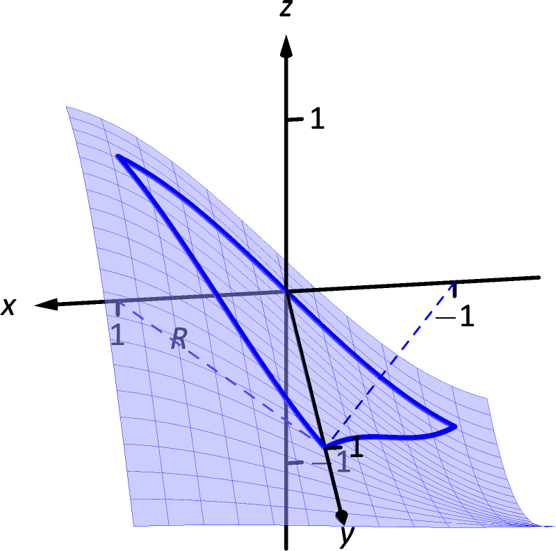Figure 14.2.6: Finding the signed volume under a surface in Example 14.2.3.

SolutionIf we attempt to integrate using an iterated integral with the order $dy\ dx$ , note how there are two upper bounds on $R$ meaning we’ll need to use two iterated integrals. We would need to split the triangle into two regions along the $y$ -axis, then use Theorem 14.2.3, part 5.

Instead, let’s use the order $dx\ dy$ . The curves bounding $x$ are $y-1\leq x\leq 1-y$ ; the bounds on $y$ are $0\leq y\leq 1$ . This gives us:

	$\displaystyle\iint_{R}f(x,y)\ dA$	$\displaystyle=\int_{0}^{1}\int_{y-1}^{1-y}\sin x\cos y\ dx\ dy$
		$\displaystyle=\int_{0}^{1}\left.\Big{(}-\cos x\cos y\Big{)}\right\|_{y-1}^{1-y}dy$
		$\displaystyle=\int_{0}^{1}\cos y\Big{(}-\cos(1-y)+\cos(y-1)\Big{)}dy.$

Recall that the cosine function is an even function; that is, $\cos x=\cos(-x)$ . Therefore, from the last integral above, we have $\cos(y-1)=\cos(1-y)$ . Thus the integrand simplifies to 0, and we have

	$\displaystyle\iint_{R}f(x,y)\ dA$	$\displaystyle=\int_{0}^{1}0\ dy$
		$\displaystyle=0.$

It turns out that over $R$ , there is just as much volume above the $x$ - $y$ plane as below (look again at Figure 14.2.6), giving a final signed volume of 0.

Example 14.2.4 Evaluating a double integral

Evaluate $\iint_{R}(4-y)\ dA$ , where $R$ is the region bounded by the parabolas $y^{2}=4x$ and $x^{2}=4y$ , graphed in Figure 14.2.7. ^†^†margin: 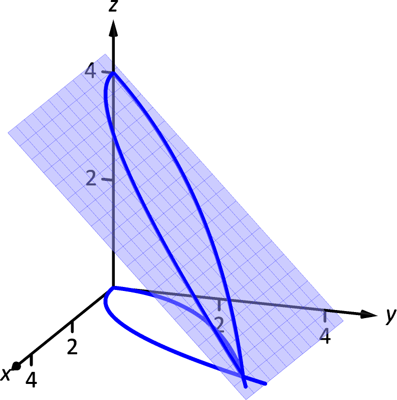Figure 14.2.7: Finding the volume under the surface in Example 14.2.4.

SolutionGraphing each curve can help us find their points of intersection. Solving analytically, the second equation tells us that $y=x^{2}/4$ . Substituting this value in for $y$ in the first equation gives us $x^{4}/16=4x$ . Solving for $x$ :

	$\displaystyle\frac{x^{4}}{16}$	$\displaystyle=4x$
	$\displaystyle x^{4}-64x$	$\displaystyle=0$
	$\displaystyle x(x^{3}-64)$	$\displaystyle=0$
	$\displaystyle x$	$\displaystyle=0,\ 4.$

Thus we’ve found analytically what was easy to approximate graphically: the regions intersect at $(0,0)$ and $(4,4)$ , as shown in Figure 14.2.7.

We now choose an order of integration: $dy\ dx$ or $dx\ dy$ ? Either order works; since the integrand does not contain $x$ , choosing $dx\ dy$ might be simpler — at least, the first integral is very simple.

Thus we have the following “curve to curve, point to point” bounds: $y^{2}/4\leq x\leq 2\sqrt{y}$ , and $0\leq y\leq 4$ .

	$\displaystyle\iint_{R}(4-y)\ dA$	$\displaystyle=\int_{0}^{4}\int_{y^{2}/4}^{2\sqrt{y}}(4-y)\ dx\ dy$
		$\displaystyle=\int_{0}^{4}\big{(}x(4-y)\big{)}\Big{\|}_{y^{2}/4}^{2\sqrt{y}}dy$
		$\displaystyle=\int_{0}^{4}\Big{(}\big{(}2\sqrt{y}-\frac{y^{2}}{4}\big{)}\big{(% }4-y)\Big{)}\ dy=\int_{0}^{4}\Big{(}\frac{y^{3}}{4}-y^{2}-2y^{3/2}+8y^{1/2}% \Big{)}\ dy$
		$\displaystyle=\left.\left(\frac{y^{4}}{16}-\frac{y^{3}}{3}-\frac{4y^{5/2}}{5}+% \frac{16y^{3/2}}{3}\right)\right\|_{0}^{4}$
		$\displaystyle=\frac{176}{15}=11.7\overline{3}.$

The signed volume under the surface $f$ is about 11.7 cubic units.

In the previous section we practiced changing the order of integration of a given iterated integral, where the region $R$ was not explicitly given. Changing the bounds of an integral is more than just an test of understanding. Rather, there are cases where integrating in one order is really hard, if not impossible, whereas integrating with the other order is feasible.

Example 14.2.5 Changing the order of integration

Rewrite the iterated integral $\displaystyle\int_{0}^{3}\int_{y}^{3}e^{-x^{2}}\ dx\ dy$ with the order $dy\ dx$ . Comment on the feasibility to evaluate each integral.

SolutionOnce again we make a sketch of the region over which we are integrating to facilitate changing the order. The bounds on $x$ are from $x=y$ to $x=3$ ; the bounds on $y$ are from $y=0$ to $y=3$ . These curves are sketched in Figure 14.2.8, enclosing the region $R$ .

^†^†margin: Figure 14.2.8: Determining the region

R

determined by the bounds of integration in Example 14.2.5.

To change the bounds, note that the curves bounding $y$ are $y=0$ up to $y=x$ ; the triangle is enclosed between $x=0$ and $x=3$ . Thus the new bounds of integration are $0\leq y\leq x$ and $0\leq x\leq 3$ , giving the iterated integral $\displaystyle\int_{0}^{3}\int_{0}^{x}e^{-x^{2}}\ dy\ dx$ .

How easy is it to evaluate each iterated integral? Consider the order of integrating $dx\ dy$ , as given in the original problem. The first indefinite integral we need to evaluate is $\int e^{-x^{2}}\ dx$ ; we have stated before (see Section 8.7) that this integral cannot be evaluated in terms of elementary functions. We are stuck.

Changing the order of integration makes a big difference here. In the second iterated integral, we are faced with $\int e^{-x^{2}}\ dy$ ; integrating with respect to $y$ gives us $ye^{-x^{2}}+C$ , and the first definite integral evaluates to

\int_{0}^{x}e^{-x^{2}}\ dy=xe^{-x^{2}}.

^†^†margin:

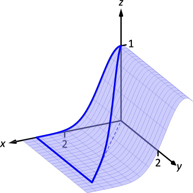Figure 14.2.9: Showing the surface

f

defined in Example 14.2.5 over its region

R

Thus

\int_{0}^{3}\int_{0}^{x}e^{-x^{2}}\ dy\ dx=\int_{0}^{3}\Big{(}xe^{-x^{2}}\Big{% )}dx.

This last integral is easy to evaluate with substitution, giving a final answer of $\frac{1}{2}(1-e^{-9})$ . Figure 14.2.9 shows the surface over $R$ .

In short, evaluating one iterated integral is impossible; the other iterated integral is relatively simple.

Definition 5.4.1 defines the average value of a single-variable function $f(x)$ on the interval $[a,b]$ as

\text{average value of $f(x)$ on $[a,b]$}=\frac{1}{b-a}\int_{a}^{b}f(x)\ dx;

that is, it is the “area under $f$ over an interval divided by the length of the interval.” We make an analogous statement here: the average value of $z=f(x,y)$ over a region $R$ is the volume under $f$ over $R$ divided by the area of $R$ .

Definition 14.2.2 The Average Value of $f$ on $R$

Let $z=f(x,y)$ be a continuous function defined over a closed region $R$ in the $x$ - $y$ plane. The average value of $f$ on $R$ is

\text{average value of $f$ on $R$}=\frac{\displaystyle\iint_{R}f(x,y)\ dA}{% \displaystyle\iint_{R}\ dA}.

Example 14.2.6 Finding average value of a function over a region $R$

Find the average value of $f(x,y)=4-y$ over the region $R$ , which is bounded by the parabolas $y^{2}=4x$ and $x^{2}=4y$ . Note: this is the same function and region as used in Example 14.2.4.

SolutionIn Example 14.2.4 we found

\iint_{R}f(x,y)\ dA=\int_{0}^{4}\int_{y^{2}/4}^{2\sqrt{y}}(4-y)\ dx\ dy=\frac{% 176}{15}.

We find the area of $R$ by computing $\iint_{R}\ dA$ :

\iint_{R}\ dA=\int_{0}^{4}\int_{y^{2}/4}^{2\sqrt{y}}\ dx\ dy=\frac{16}{3}.

^†^†margin:

Figure 14.2.10: Finding the average value of

f

in Example 14.2.6.

Dividing the volume under the surface by the area gives the average value:

\text{average value of $f$ on $R$}=\frac{176/15}{16/3}=\frac{11}{5}=2.2.

While the surface, as shown in Figure 14.2.10, covers $z$ -values from $z=0$ to $z=4$ , the “average” $z$ -value on $R$ is 2.2.

The previous section introduced the iterated integral in the context of finding the area of plane regions. This section has extended our understanding of iterated integrals; now we see they can be used to find the signed volume under a surface.

This new understanding allows us to revisit what we did in the previous section. Given a region $R$ in the plane, we computed $\iint_{R}1\ dA$ ; again, our understanding at the time was that we were finding the area of $R$ . However, we can now view the function $z=1$ as a surface, a flat surface with constant $z$ -value of 1. The double integral $\iint_{R}1\ dA$ finds the volume, under $z=1$ , over $R$ , as shown in Figure 14.2.11. Basic geometry tells us that if the base of a general right cylinder has area $A$ , its volume is $A\cdot h$ , where $h$ is the height. In our case, the height is 1. We were “actually” computing the volume of a solid, though we interpreted the number as an area.

^†^†margin:

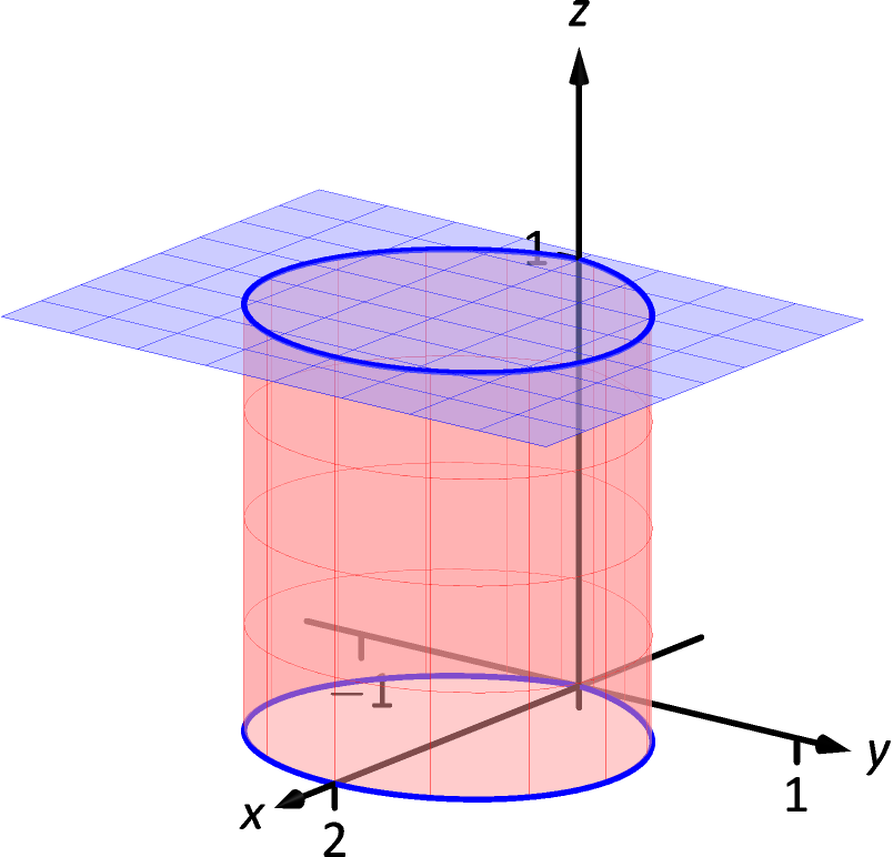Figure 14.2.11: Showing how an iterated integral used to find area also finds a certain volume.

The next section extends our abilities to find “volumes under surfaces.” Currently, some integrals are hard to compute because either the region $R$ we are integrating over is hard to define with rectangular curves, or the integrand itself is hard to deal with. Some of these problems can be solved by converting everything into polar coordinates.

Exercises 14.2

Terms and Concepts

1.

An integral can be interpreted as giving the signed area over an interval; a double integral can be interpreted as giving the signed over a region.
2.

Explain why the following statement is false: “Fubini’s Theorem states that $\displaystyle\int_{a}^{b}\int_{g_{1}(x)}^{g_{2}(x)}f(x,y)\ dy\ dx=\int_{a}^{b}% \int_{g_{1}(y)}^{g_{2}(y)}f(x,y)\ dx\ dy$ .”
3.
Explain why if $f(x,y)>0$ over a region $R$ , then $\displaystyle\iint_{R}f(x,y)\ dA>0$ .
4.

If $\displaystyle\iint_{R}f(x,y)\ dA=\iint_{R}g(x,y)\ dA$ , does this imply $f(x,y)=g(x,y)$ ?

Problems

In Exercises 5–10,

(a)

Evaluate the given iterated integral, and
(b)

rewrite the integral using the other order of integration.

5.

$\displaystyle\int_{1}^{2}\int_{-1}^{1}\left(\frac{x}{y}+3\right)\ dx\ dy$
6.

$\displaystyle\int_{-\pi/2}^{\pi/2}\int_{0}^{\pi}\left(\sin x\cos y\right)\ dx% \ dy$
7.

$\displaystyle\int_{0}^{4}\int_{0}^{-x/2+2}\left(3x^{2}-y+2\right)\ dy\ dx$
8.

$\displaystyle\int_{1}^{3}\int_{y}^{3}\left(x^{2}y-xy^{2}\right)\ dx\ dy$
9.

$\displaystyle\int_{0}^{1}\int_{-\sqrt{1-y}}^{\sqrt{1-y}}\left(x+y+2\right)\ dx% \ dy$
10.

$\displaystyle\int_{0}^{9}\int_{y/3}^{\sqrt{y}}\left(xy^{2}\right)\ dx\ dy$

In Exercises 11–18:

(a)

Sketch the region $R$ given by the problem.
(b)

Set up the iterated integrals, in both orders, that evaluate the given double integral for the described region $R$ .
(c)

Evaluate one of the iterated integrals to find the signed volume under the surface $z=f(x,y)$ over the region $R$ .

11.

$\displaystyle\iint_{R}x^{2}y\ dA$ , where $R$ is bounded by $y=\sqrt{x}$ and $y=x^{2}$ .
12.

$\displaystyle\iint_{R}x^{2}y\ dA$ , where $R$ is bounded by $y=\sqrt[3]{x}$ and $y=x^{3}$ .
13.

$\displaystyle\iint_{R}x^{2}-y^{2}\ dA$ , where $R$ is the rectangle with corners $(-1,-1)$ , $(1,-1)$ , $(1,1)$ and $(-1,1)$ .
14.

$\displaystyle\iint_{R}ye^{x}\ dA$ , where $R$ is bounded by $x=0$ , $x=y^{2}$ and $y=1$ .
15.

$\displaystyle\iint_{R}\big{(}6-3x-2y\big{)}\ dA$ , where $R$ is bounded by $x=0$ , $y=0$ and $3x+2y=6$ .
16.

$\displaystyle\iint_{R}e^{y}\ dA$ , where $R$ is bounded by $y=\ln x$ and

$\displaystyle y=\frac{1}{e-1}(x-1)$ .
17.

$\displaystyle\iint_{R}\big{(}x^{3}y-x\big{)}\ dA$ , where $R$ is the half disk $x^{2}+y^{2}\leq 9$ in the first and second quadrants.
18.

$\displaystyle\iint_{R}\big{(}4-3y\big{)}\ dA$ , where $R$ is bounded by $y=0$ , $y=x/e$ and $y=\ln x$ .

In Exercises 19–22, state why it is difficult/impossible to integrate the iterated integral in the given order of integration. Change the order of integration and evaluate the new iterated integral.

19.

$\displaystyle\int_{0}^{4}\int_{y/2}^{2}e^{x^{2}}\ dx\ dy$
20.

$\displaystyle\int_{0}^{\sqrt{\pi/2}}\int_{x}^{\sqrt{\pi/2}}\cos\big{(}y^{2}% \big{)}\ dy\ dx$
21.

$\displaystyle\int_{0}^{1}\int_{y}^{1}\frac{2y}{x^{2}+y^{2}}\ dx\ dy$
22.

$\displaystyle\int_{-1}^{1}\int_{1}^{2}\frac{x\tan^{2}y}{1+\ln y}\ dy\ dx$

In Exercises 23–26, find the average value of $f$ over the region $R$ . Notice how these functions and regions are related to the iterated integrals given in Exercises 5–8.

23.

$\displaystyle f(x,y)=\frac{x}{y}+3$ ; $R$ is the rectangle with opposite corners $(-1,1)$ and $(1,2)$ .
24.

$\displaystyle f(x,y)=\sin x\cos y$ ; $R$ is bounded by $x=0$ , $x=\pi$ , $y=-\pi/2$ and $y=\pi/2$ .
25.

$\displaystyle f(x,y)=3x^{2}-y+2$ ; $R$ is bounded by the lines $y=0$ , $y=2-x/2$ and $x=0$ .
26.

$\displaystyle f(x,y)=x^{2}y-xy^{2}$ ; $R$ is bounded by $y=x$ , $y=1$ and $x=3$ .

14.2 Double Integration and Volume

Definition 14.2.1 Double Integral, Signed Volume

Theorem 14.2.1 Double Integrals and Signed Volume

Theorem 14.2.2 Fubini’s Theorem

Example 14.2.1 Evaluating a double integral

Example 14.2.2 Evaluating a double integral

Key Idea 14.2.1 Double Integration Bounds

Theorem 14.2.3 Properties of Double Integrals

Example 14.2.3 Evaluating a double integral

Example 14.2.4 Evaluating a double integral

Example 14.2.5 Changing the order of integration

Definition 14.2.2 The Average Value of f on R

Example 14.2.6 Finding average value of a function over a region R

Exercises 14.2

Terms and Concepts

Problems

Definition 14.2.2 The Average Value of $f$ on $R$

Example 14.2.6 Finding average value of a function over a region $R$