3 The Graphical Behavior of Functions 3.4 Concavity and the Second Derivative 4 Applications of the Derivative

3.5 Curve Sketching

We have been learning how we can understand the behavior of a function based on its first and second derivatives. While we have been treating the properties of a function separately (increasing and decreasing, concave up and concave down, etc.), we combine them here to produce an accurate graph of the function without plotting lots of extraneous points.

Why bother? Graphing utilities are very accessible, whether on a computer, a hand-held calculator, or a smartphone. These resources are usually very fast and accurate. We will see that our method is not particularly fast — it will require time (but it is not hard). So again: why bother?

^†^†margin: Figure 3.5.1: Demonstrating the 4 ways that concavity interacts with increasing / decreasing, along with the relationships with the first and second derivatives. Λ

We are attempting to understand the behavior of a function $f$ based on the information given by its derivatives. While all of a function’s derivatives relay information about it, it turns out that “most” of the behavior we care about is explained by $f\,^{\prime}$ and $f\,^{\prime\prime}$ . Understanding the interactions between the graph of $f$ and $f\,^{\prime}$ and $f\,^{\prime\prime}$ is important and is illustrated in Figure 3.5.1. To gain this understanding, one might argue that all that is needed is to look at lots of graphs. This is true to a point, but is somewhat similar to stating that one understands how an engine works after looking only at pictures. It is true that the basic ideas will be conveyed, but “hands-on” access increases understanding.

The following Key Idea summarizes what we have learned so far that is applicable to sketching graphs of functions and gives a framework for putting that information together. It is followed by several examples.

Key Idea 3.5.1 Curve Sketching

To produce an accurate sketch a given function $f$ , consider the following steps.

(a)

Find the domain of $f$ . Generally, we assume that the domain is the entire real line then find restrictions, such as where a denominator is 0 or where negatives appear under the radical.
(b)

Find the location of any vertical asymptotes of $f$ (usually done in conjunction with the previous step).
(c)

Find the $x$ and $y$ -intercepts of $f$ , and any symmetry.
(d)

Consider the limits $\displaystyle\lim_{x\to-\infty}f(x)$ and $\displaystyle\lim_{x\to\infty}f(x)$ to determine the end behavior of the function.
(e)

Find the critical points of $f$ .
(f)

Find the possible points of inflection of $f$ .
(g)

Create a number line that includes all critical points, possible points of inflection, and locations of vertical asymptotes. For each interval created, determine whether $f$ is increasing or decreasing, concave up or down.
(h)

Evaluate $f$ at each critical point and possible point of inflection. Plot these points on a set of axes. Connect these points with curves exhibiting the proper concavity. Sketch asymptotes and $x$ and $y$ -intercepts where applicable.

Watch the video:
Summary of Curve Sketching — Example 2, Part 1 of 4 from https://youtu.be/DMYUsv8ZaoY

Example 3.5.1 Curve sketching

Use Key Idea 3.5.1 to sketch $f(x)=3x^{3}-10x^{2}+4x+10$ .

SolutionWe follow the steps outlined in the Key Idea.

(a)

The domain of $f$ is the entire real line; there are no values $x$ for which $f(x)$ is not defined.
(b)

There are no vertical asymptotes.
(c)

We see that $f(0)=10$ , and $f$ does not appear to factor easily (so we skip finding the roots). It has no symmetry.
(d)

We determine the end behavior using limits as $x$ approaches $\pm$ infinity.

$\lim_{x\to-\infty}f(x)=-\infty\qquad\lim_{x\to\infty}f(x)=\infty.$

We do not have any horizontal asymptotes.
(e)

Find the critical points of $f$ . We compute $f\,^{\prime}(x)=9x^{2}-20x+4=(9x-2)(x-2)$ , so that $x=\frac{2}{9},2$ .
(f)

Find the possible points of inflection of $f$ . We see $f\,^{\prime\prime}(x)=18x-20$ , so that

$f\,^{\prime\prime}(x)=0\Rightarrow x=10/9\approx 1.111.$
(g)

We place the values $x=\frac{2}{9},\frac{10}{9},2$ on a number line. We mark each subinterval as increasing or decreasing, concave up or down, using the techniques used in Sections 3.3 and 3.4.

^†^†margin: (a) (b) Figure 3.5.2: Sketching $f$ in Example 3.5.1. Λ
(h)

We plot the appropriate points on axes as shown in Figure 3.5.2(a) and connect the points with the proper concavity. Our curve crosses the $y$ axis at $y=10$ and crosses the $x$ axis near $x=-0.75$ . In Figure 3.5.2(b) we show a graph of $f$ drawn with a computer program, verifying the accuracy of our sketch.

Example 3.5.2 Curve sketching

Sketch $\displaystyle f(x)=\frac{x^{2}-x-2}{x^{2}-x-6}$ .

SolutionWe again follow the steps outlined in Key Idea 3.5.1.

(a)

In determining the domain, we assume it is all real numbers and look for restrictions. We find that at $x=-2$ and $x=3$ , $f(x)$ is not defined. So the domain of $f$ is $D=\{\text{real numbers }x\ |\ x\neq-2,3\}$ .
(b)

The vertical asymptotes of $f$ are at $x=-2$ and $x=3$ , the places where $f$ is undefined. We see that $\displaystyle\lim_{x\to-2^{-}}f(x)=\infty$ , $\displaystyle\lim_{x\to-2^{+}}f(x)=-\infty$ , $\displaystyle\lim_{x\to 3^{-}}f(x)=-\infty$ , and $\displaystyle\lim_{x\to 3^{+}}f(x)=\infty$ .
(c)

We see that $f(0)=\frac{1}{3}$ and that $f(x)=0$ when $0=x^{2}-x-2=(x-2)(x+1)$ so that $x=-1,2$ . There is no symmetry.
(d)

There is a horizontal asymptote of $y=1$ , as both $\displaystyle\lim_{x\to-\infty}f(x)=1$ and $\displaystyle\lim_{x\to\infty}f(x)=1$ . (Either one would be sufficient to give the horizontal asymptote.)
(e)

To find the critical points of $f$ , we first find $f\,^{\prime}(x)$ . Using the Quotient Rule, we find

$f\,^{\prime}(x)=\frac{-8x+4}{(x^{2}-x-6)^{2}}=\frac{-8x+4}{(x-3)^{2}(x+2)^{2}}.$

$f\,^{\prime}(x)=0$ when $x=1/2$ , and $f\,^{\prime}$ is undefined when $x=-2,3$ . Since $f\,^{\prime}$ is undefined only when $f$ is, these are not critical points. The only critical point is $x=1/2$ .
(f)

To find the possible points of inflection, we find $f\,^{\prime\prime}(x)$ , again employing the Quotient Rule:

$f\,^{\prime\prime}(x)=\frac{24x^{2}-24x+56}{(x-3)^{3}(x+2)^{3}}.$

We find that $f\,^{\prime\prime}(x)$ is never 0 (setting the numerator equal to 0 and solving for $x$ , we find the only roots to this quadratic are imaginary) and $f\,^{\prime\prime}$ is undefined when $x=-2,3$ . Thus concavity will possibly only change at $x=-2$ and $x=3$ (although these are not inflection points, since $f$ is not defined there). ^†^†margin: (a) (b) Figure 3.5.3: Sketching $f$ in Example 3.5.2. Λ
(g)

We place the values $x=1/2$ , $x=-2$ and $x=3$ on a number line. We mark in each interval whether $f$ is increasing or decreasing, concave up or down. We see that $f$ has a relative maximum at $x=1/2$ ; concavity changes only at the vertical asymptotes.
(h)

In Figure 3.5.3(a), we plot the points from the number line on a set of axes and connect the points with the appropriate concavity. We also show $f$ crossing the $x$ axis at $x=-1$ and $x=2$ . Figure 3.5.3(b) shows a computer generated graph of $f$ , which verifies the accuracy of our sketch.

Example 3.5.3 Curve sketching

Sketch $\displaystyle f(x)=\frac{5(x-2)(x+1)}{x^{2}+2x+4}$ .

SolutionWe again follow Key Idea 3.5.1.

(a)

We assume that the domain of $f$ is all real numbers and consider restrictions. The only restrictions come when the denominator is 0, but this never occurs. Therefore the domain of $f$ is all real numbers, $\mathbb{R}$ .
(b)

There are no vertical asymptotes.
(c)

We see that $f(0)=-\dfrac{5}{2}$ and that $f(x)=0$ when $x=-1,2$ .
(d)

We have a horizontal asymptote of $y=5$ , as

$\lim_{x\to\pm\infty}f(x)=\lim_{x\to\pm\infty}\frac{5(1-\frac{2}{x})(1+\frac{1}% {x})}{1+\frac{2}{x}+\frac{4}{x^{2}}}=5.$
(e)

We find the critical points of $f$ by setting $f\,^{\prime}(x)=0$ and solving for $x$ . We find

$f\,^{\prime}(x)=\frac{15x(x+4)}{(x^{2}+2x+4)^{2}}\quad\Rightarrow\quad f\,^{% \prime}(x)=0\text{ when }\ x=-4,0.$
(f)

We find the possible points of inflection by solving $f\,^{\prime\prime}(x)=0$ for $x$ . We find

$f\,^{\prime\prime}(x)=-\frac{30x^{3}+180x^{2}-240}{(x^{2}+2x+4)^{3}}.$

The cubic in the numerator does not factor very “nicely.” We instead approximate the roots at $x=-5.759$ , $x=-1.305$ and $x=1.064$ .
(g)

We place the critical points and possible inflection points on a number line and mark each interval as increasing/decreasing, concave up/down appropriately.
(h)

In Figure 3.5.4(a) we plot the significant points from the number line as well as the two roots of $f$ , $x=-1$ and $x=2$ , and connect the points with the appropriate concavity. Figure 3.5.4(b) shows a computer generated graph of $f$ , affirming our results (but the top left was slightly off). ^†^†margin: (a) (b) Figure 3.5.4: Sketching $f$ in Example 3.5.3. Λ

In each of our examples, we found a few, significant points on the graph of $f$ that corresponded to changes in increasing/decreasing or concavity. We connected these points with curves, and finished by showing a very accurate, computer generated graph.

Why are computer graphics so good? It is not because computers are “smarter” than we are. Rather, it is largely because computers are much faster at computing than we are. In general, computers graph functions much like most students do when first learning to draw graphs: they plot equally spaced points, then connect the dots using lines. By using lots of points, the connecting lines are short and the graph looks smooth.

This does a fine job of graphing in most cases (in fact, this is the method used for many graphs in this text). However, in regions where the graph is very “curvy,” this can generate noticeable sharp edges on the graph unless a large number of points are used. High quality computer algebra systems, such as Mathematica, use special algorithms to plot lots of points only where the graph is “curvy.”

In Figure 3.5.5, a graph of $y=\sin x$ is given, generated by Mathematica. The small points represent each of the places Mathematica sampled the function. Notice how at the “bends” of $\sin x$ , lots of points are used; where $\sin x$ is relatively straight, fewer points are used. (Many points are also used at the endpoints to ensure the “end behavior” is accurate.)

Figure 3.5.5: A graph of

y=\sin x

generated by Mathematica.

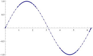
How does Mathematica know where the graph is “curvy”? Calculus. When we study curvature in a later chapter, we will see how the first and second derivatives of a function work together to provide a measurement of “curviness.” Mathematica employs algorithms to determine regions of “high curvature” and plots extra points there.

Again, the goal of this section is not “How to graph a function when there is no computer to help.” Rather, the goal is “Understand that the shape of the graph of a function is largely determined by understanding the behavior of the function at a few key places.” In Example 3.5.3, we were able to accurately sketch a complicated graph using only 5 points and knowledge of asymptotes!

There are many applications of our understanding of derivatives beyond curve sketching. The next chapter explores some of these applications, demonstrating just a few kinds of problems that can be solved with a basic knowledge of differentiation.

Exercises 3.5

Terms and Concepts

1.

Why is sketching curves by hand beneficial even though technology is readily available?
2.

T/F: When sketching graphs of functions, it is useful to find the critical points.
3.

T/F: When sketching graphs of functions, it is useful to find the possible points of inflection.
4.

T/F: When sketching graphs of functions, it is useful to find the horizontal and vertical asymptotes.

Problems

5.
Given the graph of $f$ , identify the concavity of $f$ , its inflection points, its regions of increasing and decreasing, and its relative extrema.
6.
Given the graph of $f\,^{\prime}$ , identify the concavity of $f$ , its inflection points, its regions of increasing and decreasing, and its relative extrema.

In Exercises 7–12., practice using Key Idea 3.5.1 by applying the principles to the given functions with familiar graphs.

7.

$f(x)=2x+4$
8.

$f(x)=-x^{2}+1$
9.

$f(x)=\sin x$
10.

$f(x)=e^{x}$
11.

$\displaystyle f(x)=\frac{1}{x}$
12.

$\displaystyle f(x)=\frac{1}{x^{2}}$

In Exercises 13–46., sketch a graph of the given function using Key Idea 3.5.1. Show all work; check your answer with technology.

13.

$f(x)=x^{3}-2x^{2}+4x+1$
14.

$f(x)=-x^{3}+5x^{2}-3x+2$
15.

$f(x)=x^{3}+3x^{2}+3x+1$
16.

$f(x)=x^{3}-x^{2}-x+1$
17.

$f(x)=(x-2)\ln(x-2)$
18.

$f(x)=(x-2)^{2}\ln(x-2)$
19.

$f(x)=\dfrac{x^{2}-4}{x^{2}}$
20.

$f(x)=\dfrac{x^{2}-4x+3}{x^{2}-6x+8}$
21.

$f(x)=x+\sin x$ on $[0,2\pi]$ .
22.

$f(x)=\dfrac{x^{2}-2x+1}{x^{2}-6x+8}$
23.

$f(x)=x\sqrt{x+1}$
24.

$f(x)=x^{2}e^{x}$
25.

$f(x)=\sin x\cos x$ on $[-\pi,\pi]$
26.

$f(x)=(x-3)^{2/3}+2$
27.

$f(x)=\dfrac{(x-1)^{2/3}}{x}$
28.

$\displaystyle f(x)=\sqrt{\frac{x}{x-5}}$
29.

$f(x)=\sec x-2\cos x$ on $[0,2\pi]$ .
30.

$f(x)=x\sqrt{2-x^{2}}$
31.

$f(x)=\dfrac{x}{\sqrt{x^{2}-1}}$
32.

$f(x)=x^{5/3}-5x^{2/3}$
33.

$f(x)=\dfrac{\sin x}{2+\cos x}$ on $[0,2\pi]$ .
34.

$f(x)=\dfrac{x}{x^{2}+3}$
35.
$f(x)=\dfrac{4x^{2}-4x+1}{4x^{2}-12x+9}$ Hint: $f(x)$ can be simplified in a variety of ways. Use whichever simplification works best for your current task.
36.

$y=\sqrt{x^{2}+x}-x$
37.

$y=x+\cos x$
38.

$y=x\tan x$ on $(-\frac{\pi}{2},\frac{\pi}{2})$
39.

$y=\sin x+\sqrt{3}\cos x$ on $[-2\pi,2\pi]$
40.

$y=\csc x-2\sin x$ on $(0,\pi)$
41.

$f(x)=\dfrac{3}{x^{2}+4}$
42.

$f(x)=\dfrac{3}{x^{2}-4}$
43.

$f(x)=\dfrac{x}{x^{2}+4}$
44.

$f(x)=\dfrac{x}{x^{2}-4}$
45.

$f(x)=\dfrac{x}{x-4}$
46.

$f(x)=\dfrac{(x-1)^{2}}{x^{2}+1}$

In Exercises 47–52., sketch the graph of a function that satisfies all of the given conditions.

47.
$f\,^{\prime}(0)=f\,^{\prime}(2)=f\,^{\prime}(4)=0$ , $f\,^{\prime}(x)>0$ if $x<0$ or $2<x<4$ , $f\,^{\prime}(x)<0$ if $0<x<2$ or $x>4$ , $f\,^{\prime\prime}(x)>0$ if $1<x<3$ , $f\,^{\prime\prime}(x)<0$ if $x<1$ or $x>4$
48.
$f\,^{\prime}(5)=0$ , $f\,^{\prime}(x)<0$ when $x<5$ , $f\,^{\prime}(x)>0$ if $x>5$ , $f\,^{\prime\prime}(2)=0$ , $f\,^{\prime\prime}(8)=0$ , $f\,^{\prime\prime}(x)<0$ if $x<2$ or $x>8$ , $f\,^{\prime\prime}(x)>0$ if $2<x<8$
49.
$f(0)=0$ , $f\,^{\prime}(-2)=f\,^{\prime}(1)=f\,^{\prime}(9)=0$ , $\displaystyle\lim_{x\to\infty}f(x)=0$ , $\displaystyle\lim_{x\to 6}f(x)=-\infty$ , $f\,^{\prime}(x)<0$ on $(-\infty,-2),(1,6),(9,\infty)$ , $f\,^{\prime}(x)>0$ on $(-2,1),(6,9)$ , $f\,^{\prime\prime}(x)>0$ on $(-\infty,0),(12,\infty)$ , $f\,^{\prime\prime}(x)<0$ on $(0,6),(6,12)$
50.
$f$ is odd, $f\,^{\prime}(x)<0$ on $(0,2)$ , $f\,^{\prime}(x)>0$ on $(2,\infty)$ , $f\,^{\prime\prime}(x)>0$ on $(0,3)$ , $f\,^{\prime\prime}(x)<0$ on $(3,\infty)$ , $\displaystyle\lim_{x\to\infty}f(x)=-2$
51.
concave up on $(-\infty,-1)$ , $(1,\infty)$ ; concave down on $(-1,1)$ ; increasing on $(-\infty,0)$ ; and decreasing on $(0,\infty)$ .
52.
$\displaystyle\lim_{x\to-\infty}f(x)=1$ , $\displaystyle\lim_{x\to 3^{-}}f(x)=\infty$ , $\displaystyle\lim_{x\to\infty}f(x)=-1$ , $\displaystyle\lim_{x\to 3^{+}}f(x)=-\infty$ ; $f\,^{\prime}(x)>0$ on $(-\infty,-2)$ , $(-1,0)$ , $(2,3)$ , $(3,\infty)$ ; $f\,^{\prime}(x)<0$ on $(-2,-1)$ , $(0,2)$ ; $f\,^{\prime\prime}(x)>0$ on $(-\infty,-3)$ , $(1,3)$ ; and $f\,^{\prime\prime}(x)<0$ on $(-3,-1)$ , $(-1,1)$ , $(3,\infty)$ .

In Exercises 53–56., a function with the parameters $a$ and $b$ are given. Describe the critical points and possible points of inflection of $f$ in terms of $a$ and $b$ .

53.

$\displaystyle f(x)=\frac{a}{x^{2}+b^{2}}$
54.

$f(x)=ax^{2}+bx+1$
55.

$\displaystyle f(x)=\sin(ax+b)$
56.

$\displaystyle f(x)=(x-a)(x-b)$

57.

Given $x^{2}+y^{2}=1$ , use implicit differentiation to find $\dfrac{\operatorname{d}\!y}{\operatorname{d}\!x}$ and $\dfrac{\operatorname{d}\!^{2}y}{\operatorname{d}\!x^{2}}$ . Use this information to justify the sketch of the unit circle.