12 Vector Valued Functions Chapter Introduction 12.2 Calculus and Vector-Valued Functions

12.1 Vector-Valued Functions

We are very familiar with real valued functions, that is, functions whose output is a real number. This section introduces vector-valued functions — functions whose output is a vector.

Definition 12.1.1 Vector-Valued Functions

A vector-valued function is a function of the form

\vec{r}(t)=\left\langle\,f(t),g(t)\,\right\rangle\quad\text{or}\quad\vec{r}(t)% =\left\langle\,f(t),g(t),h(t)\,\right\rangle,

where $f$ , $g$ and $h$ are real valued functions.

The domain of $\vec{r}$ is the set of all values of $t$ for which $\vec{r}(t)$ is defined. The range of $\vec{r}$ is the set of all possible output vectors $\vec{r}(t)$ .

Evaluating and Graphing Vector-Valued Functions

^†^†margin: (a) (b) Figure 12.1.1: Sketching the graph of a vector-valued function.

Evaluating a vector-valued function at a specific value of $t$ is straightforward; simply evaluate each component function at that value of $t$ . For instance, if $\vec{r}(t)=\left\langle t^{2},t^{2}+t-1\right\rangle$ , then $\vec{r}(-2)=\left\langle 4,1\right\rangle$ . We can sketch this vector, as is done in Figure 12.1.1(a). Plotting lots of vectors is cumbersome, though, so generally we do not sketch the whole vector but just the terminal point. The graph of a vector-valued function is the set of all terminal points of $\vec{r}(t)$ , where the initial point of each vector is always the origin. In Figure 12.1.1(b) we sketch the graph of $\vec{r}$ ; we can indicate individual points on the graph with their respective vector, as shown.

Vector-valued functions are closely related to parametric equations of graphs. While in both methods we plot points $\big{(}x(t),y(t)\big{)}$ or $\big{(}x(t),y(t),z(t)\big{)}$ to produce a graph, in the context of vector-valued functions each such point represents a vector. The implications of this will be more fully realized in the next section as we apply calculus ideas to these functions.

Watch the video:
Domain of a Vector-Valued Function from https://youtu.be/Djtttm0C7zA

^†^†margin:

t

t^{3}-t

\displaystyle\frac{1}{t^{2}+1}

-2

-6

1/5

-1

0 1/2 0 0 1 1 0 1/2 2 6 1/5 (a) (b) Figure 12.1.2: Sketching the vector-valued function of Example 12.1.1.

Example 12.1.1 Graphing vector-valued functions

Graph $\displaystyle\vec{r}(t)=\left\langle t^{3}-t,\frac{1}{t^{2}+1}\right\rangle$ , for $-2\leq t\leq 2$ . Sketch $\vec{r}(-1)$ and $\vec{r}(2)$ .

SolutionWe start by making a table of $t$ , $x$ and $y$ values as shown in Figure 12.1.2(a). Plotting these points gives an indication of what the graph looks like. In Figure 12.1.2(b), we indicate these points and sketch the full graph. We also highlight $\vec{r}(-1)$ and $\vec{r}(2)$ on the graph.

^†^†margin:

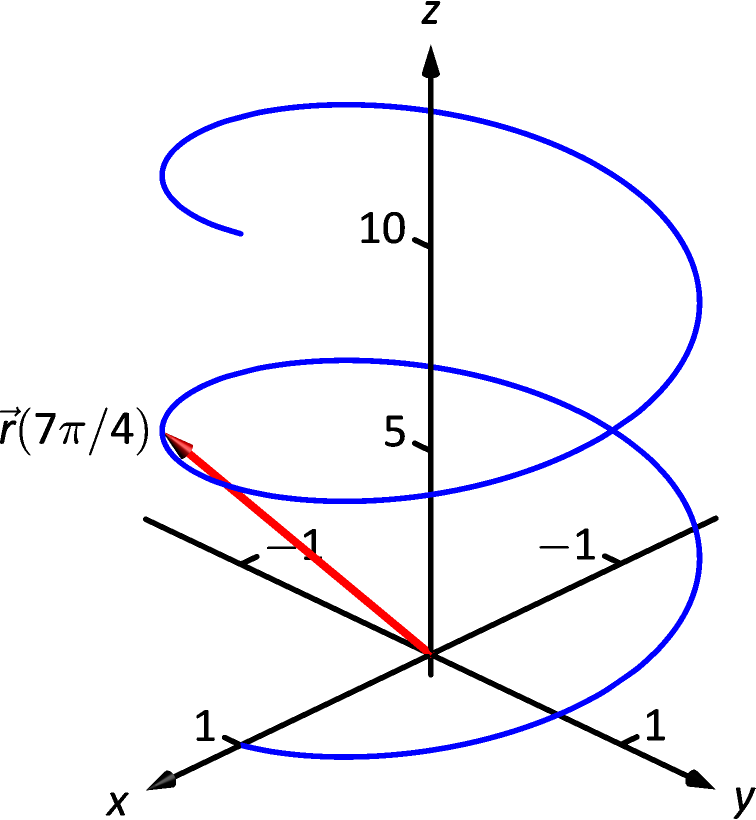Figure 12.1.3: Viewing a vector-valued function, and its value at one point.

Example 12.1.2 Graphing vector-valued functions.

Graph $\vec{r}(t)=\left\langle\cos t,\sin t,t\right\rangle$ for $0\leq t\leq 4\pi$ .

SolutionWe can again plot points, but careful consideration of this function is very revealing. Momentarily ignoring the third component, we see the $x$ and $y$ components trace out a circle of radius 1 centered at the origin. Noticing that the $z$ component is $t$ , we see that as the graph winds around the $z$ -axis, it is also increasing at a constant rate in the positive $z$ direction, forming a spiral. This is graphed in Figure 12.1.3. In the graph $\vec{r}(7\pi/4)=\left\langle\frac{1}{\sqrt{2}},-\frac{1}{\sqrt{2}},\frac{7\pi}% {4}\right\rangle$ is highlighted to help us understand the graph.

Example 12.1.3 Adding and scaling vector-valued functions.

Let $\vec{r}_{1}(t)=\left\langle\,0.2t,0.3t\,\right\rangle$ , $\vec{r}_{2}(t)=\left\langle\,\cos t,\sin t\,\right\rangle$ and $\vec{r}(t)=\vec{r}_{1}(t)+\vec{r}_{2}(t)$ . Graph $\vec{r}_{1}(t)$ , $\vec{r}_{2}(t)$ , $\vec{r}(t)$ and $5\vec{r}(t)$ on $-10\leq t\leq 10$ .

SolutionWe can graph $\vec{r}_{1}$ and $\vec{r}_{2}$ easily by plotting points (or just using technology). Let’s think about each for a moment to better understand how vector-valued functions work.

We can rewrite $\vec{r}_{1}(t)=\left\langle\,0.2t,0.3t\,\right\rangle$ as $\vec{r}_{1}(t)=t\left\langle 0.2,0.3\right\rangle$ . That is, the function $\vec{r}_{1}$ scales the vector $\left\langle 0.2,0.3\right\rangle$ by $t$ . This scaling of a vector produces a line in the direction of $\left\langle 0.2,0.3\right\rangle$ .

We are familiar with $\vec{r}_{2}(t)=\left\langle\,\cos t,\sin t\,\right\rangle$ ; it traces out a circle, centered at the origin, of radius 1. Figure 12.1.4(a) graphs $\vec{r}_{1}(t)$ and $\vec{r}_{2}(t)$ .

^†^†margin: (a) (b) (c) Figure 12.1.4: Graphing the functions in Example 12.1.3.

Adding $\vec{r}_{1}(t)$ to $\vec{r}_{2}(t)$ produces $\vec{r}(t)=\left\langle\,\cos t+0.2t,\sin t+0.3t\,\right\rangle$ , graphed in Figure 12.1.4(b). The linear movement of the line combines with the circle to create loops that move in the direction of $\left\langle 0.2,0.3\right\rangle$ . (We encourage the reader to experiment by changing $\vec{r}_{1}(t)$ to $\left\langle 2t,3t\right\rangle$ , etc., and observe the effects on the loops.)

Multiplying $\vec{r}(t)$ by 5 scales the function by 5, producing $5\vec{r}(t)=\left\langle 5\cos t+1,5\sin t+1.5\right\rangle$ , which is graphed in Figure 12.1.4(c) along with $\vec{r}(t)$ . The new function is “5 times bigger” than $\vec{r}(t)$ . Note how the graph of $5\vec{r}(t)$ in (c) looks identical to the graph of $\vec{r}(t)$ in $(b)$ . This is due to the fact that the $x$ and $y$ bounds of the plot in $(c)$ are exactly 5 times larger than the bounds in (b).

Example 12.1.4 Adding and scaling vector-valued functions.

A cycloid is a graph traced by a point $p$ on a rolling circle, as shown in Figure 12.1.5. Find an equation describing the cycloid, where the circle has radius 1.

Figure 12.1.5: Tracing a cycloid.

SolutionThis problem is not very difficult if we approach it in a clever way. We start by letting $\vec{p}(t)$ describe the position of the point $p$ on the circle, where the circle is centered at the origin and only rotates clockwise (i.e., it does not roll). This is relatively simple given our previous experiences with parametric equations; $\vec{p}(t)=\left\langle\cos t,-\sin t\right\rangle$ .

We now want the circle to roll. We represent this by letting $\vec{c}(t)$ represent the location of the center of the circle. It should be clear that the $y$ component of $\vec{c}(t)$ should be 1; the center of the circle is always going to be 1 if it rolls on a horizontal surface.

^†^†margin: Figure 12.1.6: The cycloid in Example 12.1.4.

The $x$ component of $\vec{c}(t)$ is a linear function of $t$ : $f(t)=mt$ for some scalar $m$ . When $t=0$ , $f(t)=0$ (the circle starts centered on the $y$ -axis). When $t=2\pi$ , the circle has made one complete revolution, traveling a distance equal to its circumference, which is also $2\pi$ . This gives us a point on our line $f(t)=mt$ , the point $(2\pi,2\pi)$ . It should be clear that $m=1$ and $f(t)=t$ . So $\vec{c}(t)=\left\langle t,1\right\rangle$ .

We now combine $\vec{p}$ and $\vec{c}$ together to form the equation of the cycloid: $\vec{r}(t)=\vec{p}(t)+\vec{c}(t)=\left\langle\cos t+t,-\sin t+1\right\rangle$ , which is graphed in Figure 12.1.6.

Displacement

A vector-valued function $\vec{r}(t)$ is often used to describe the position of a moving object at time $t$ . At $t=t_{0}$ , the object is at $\vec{r}(t_{0})$ ; at $t=t_{1}$ , the object is at $\vec{r}(t_{1})$ . Knowing the locations $\vec{r}(t_{0})$ and $\vec{r}(t_{1})$ give no indication of the path taken between them, but often we only care about the difference of the locations, $\vec{r}(t_{1})-\vec{r}(t_{0})$ , the displacement.

Definition 12.1.2 Displacement

Let $\vec{r}(t)$ be a vector-valued function and let $t_{0}<t_{1}$ be values in the domain. The displacement $\vec{d}$ of $\vec{r}$ , from $t=t_{0}$ to $t=t_{1}$ , is

\vec{d}=\vec{r}(t_{1})-\vec{r}(t_{0}).

When the displacement vector is drawn with initial point at $\vec{r}(t_{0})$ , its terminal point is $\vec{r}(t_{1})$ . We think of it as the vector which points from a starting position to an ending position.

Example 12.1.5 Finding and graphing displacement vectors

Let $\vec{r}(t)=\left\langle\cos(\frac{\pi}{2}t),\sin(\frac{\pi}{2}t)\right\rangle$ . Graph $\vec{r}(t)$ on $-1\leq t\leq 1$ , and find the displacement of $\vec{r}(t)$ on this interval.

SolutionThe function $\vec{r}(t)$ traces out the unit circle, though at a different rate than the “usual” $\left\langle\cos t,\sin t\right\rangle$ parameterization. At $t_{0}=-1$ , we have $\vec{r}(t_{0})=\left\langle 0,-1\right\rangle$ ; at $t_{1}=1$ , we have $\vec{r}(t_{1})=\left\langle 0,1\right\rangle$ . The displacement of $\vec{r}(t)$ on $[-1,1]$ is thus $\vec{d}=\left\langle 0,1\right\rangle-\left\langle 0,-1\right\rangle=\left% \langle 0,2\right\rangle.$

^†^†margin: Figure 12.1.7: Graphing the displacement of a position function in Example 12.1.5.

A graph of $\vec{r}(t)$ on $[-1,1]$ is given in Figure 12.1.7, along with the displacement vector $\vec{d}$ on this interval.

Measuring displacement makes us contemplate related, yet very different, concepts. Considering the semi-circular path the object in Example 12.1.5 took, we can quickly verify that the object ended up a distance of 2 units from its initial location. That is, we can compute $\left\lVert\vec{d}\right\rVert=2$ . However, measuring distance from the starting point is different from measuring distance traveled. Being a semi-circle, we can measure the distance traveled by this object as $\pi$ units. Knowing distance from the starting point allows us to compute average rate of change.

Definition 12.1.3 Average Rate of Change

Let $\vec{r}(t)$ be a vector-valued function, where each of its component functions is continuous on its domain, and let $t_{0}<t_{1}$ . The average rate of change of $\vec{r}(t)$ on $[t_{0},t_{1}]$ is

\text{average rate of change}=\frac{\vec{r}(t_{1})-\vec{r}(t_{0})}{t_{1}-t_{0}}.

Example 12.1.6 Average rate of change

Let $\vec{r}(t)=\left\langle\cos(\frac{\pi}{2}t),\sin(\frac{\pi}{2}t)\right\rangle$ as in Example 12.1.5. Find the average rate of change of $\vec{r}(t)$ on $[-1,1]$ and on $[-1,5]$ .

SolutionWe computed in Example 12.1.5 that the displacement of $\vec{r}(t)$ on $[-1,1]$ was $\vec{d}=\left\langle 0,2\right\rangle$ . Thus the average rate of change of $\vec{r}(t)$ on $[-1,1]$ is:

\frac{\vec{r}(1)-\vec{r}(-1)}{1-(-1)}=\frac{\left\langle 0,2\right\rangle}{2}=% \left\langle 0,1\right\rangle.

We interpret this as follows: the object followed a semi-circular path, meaning it moved towards the right then moved back to the left, while climbing slowly, then quickly, then slowly again. On average, however, it progressed straight up at a constant rate of $\left\langle 0,1\right\rangle$ per unit of time.

We can quickly see that the displacement on $[-1,5]$ is the same as on $[-1,1]$ , so $\vec{d}=\left\langle 0,2\right\rangle$ . The average rate of change is different, though:

\frac{\vec{r}(5)-\vec{r}(-1)}{5-(-1)}=\frac{\left\langle 0,2\right\rangle}{6}=% \left\langle 0,1/3\right\rangle.

As it took “3 times as long” to arrive at the same place, this average rate of change on $[-1,5]$ is $1/3$ the average rate of change on $[-1,1]$ .

We considered average rates of change in Sections 1.1 and 2.1 as we studied limits and derivatives. The same is true here; in the following section we apply calculus concepts to vector-valued functions as we find limits, derivatives, and integrals. Understanding the average rate of change will give us an understanding of the derivative; displacement gives us one application of integration.

Exercises 12.1

Terms and Concepts

1.

Vector-valued functions are closely related to of graphs.
2.

When sketching vector-valued functions, technically one isn’t graphing points, but rather .
3.

It can be useful to think of as a vector that points from a starting position to an ending position.
4.

In the context of vector-valued functions, average rate of change is divided by time.

Problems

In Exercises 5–12, sketch the vector-valued function on the given interval.

5.

$\vec{r}(t)=\left\langle t^{2},t^{2}-1\right\rangle$ , for $-2\leq t\leq 2$ .
6.

$\vec{r}(t)=\left\langle t^{2},t^{3}\right\rangle$ , for $-2\leq t\leq 2$ .
7.

$\vec{r}(t)=\left\langle 1/t,1/t^{2}\right\rangle$ , for $-2\leq t\leq 2$ .
8.

$\vec{r}(t)=\left\langle\frac{1}{10}t^{2},\sin t\right\rangle$ , for $-2\pi\leq t\leq 2\pi$ .
9.

$\vec{r}(t)=\left\langle\frac{1}{10}t^{2},\sin t\right\rangle$ , for $-2\pi\leq t\leq 2\pi$ .
10.

$\vec{r}(t)=\left\langle 3\sin(\pi t),2\cos(\pi t)\right\rangle$ , on $[0,2]$ .
11.

$\vec{r}(t)=\left\langle 3\cos t,2\sin(2t)\right\rangle$ , on $[0,2\pi]$ .
12.

$\vec{r}(t)=\left\langle 2\sec t,\tan t\right\rangle$ , on $[-\pi,\pi]$ .

In Exercises 13–16, sketch the vector-valued function on the given interval in $\mathbb{R}^{3}$ . Technology may be useful in creating the sketch.

13.

$\vec{r}(t)=\left\langle 2\cos t,t,2\sin t\right\rangle$ , on $[0,2\pi]$ .
14.

$\vec{r}(t)=\left\langle 3\cos t,\sin t,t/\pi\right\rangle$ on $[0,2\pi]$ .
15.

$\vec{r}(t)=\left\langle\cos t,\sin t,\sin t\right\rangle$ on $[0,2\pi]$ .
16.

$\vec{r}(t)=\left\langle\cos t,\sin t,\sin(2t)\right\rangle$ on $[0,2\pi]$ .

In Exercises 17–20, find $\left\lVert\vec{r}(t)\right\rVert$ .

17.

$\vec{r}(t)=\left\langle t,t^{2}\right\rangle$ .
18.

$\vec{r}(t)=\left\langle 5\cos t,3\sin t\right\rangle$ .
19.

$\vec{r}(t)=\left\langle 2\cos t,2\sin t,t\right\rangle$ .
20.

$\vec{r}(t)=\left\langle\cos t,t,t^{2}\right\rangle$ .

In Exercises 21–30, create a vector-valued function whose graph matches the given description.

21.

A circle of radius 2, centered at $(1,2)$ , traced counter-clockwise once on $[0,2\pi]$ .
22.

A circle of radius 3, centered at $(5,5)$ , traced clockwise once on $[0,2\pi]$ .
23.

An ellipse, centered at $(0,0)$ with vertical major axis of length 10 and minor axis of length 3, traced once counter-clockwise on $[0,2\pi]$ .
24.

An ellipse, centered at $(3,-2)$ with horizontal major axis of length 6 and minor axis of length 4, traced once clockwise on $[0,2\pi]$ .
25.

A line through $(2,3)$ with a slope of 5.
26.

A line through $(1,5)$ with a slope of $-1/2$ .
27.

A vertically oriented helix with radius of 2 that starts at $(2,0,0)$ and ends at $(2,0,4\pi)$ after 1 revolution on $[0,2\pi]$ .
28.

A vertically oriented helix with radius of 3 that starts at $(3,0,0)$ and ends at $(3,0,3)$ after 2 revolutions on $[0,1]$ .
29.

A vertically oriented helix with radius $R$ which completes $N$ revolutions over a height of $h$ on $[0,1]$ .
30.

The intersection of the sphere $x^{2}+y^{2}+z^{2}=9$ and the plane $y=2$ on $[0,1]$ .

In Exercises 31–34, find the average rate of change of $\vec{r}(t)$ on the given interval.

31.

$\vec{r}(t)=\left\langle t,t^{2}\right\rangle$ on $[-2,2]$ .
32.

$\vec{r}(t)=\left\langle t,t+\sin t\right\rangle$ on $[0,2\pi]$ .
33.

$\vec{r}(t)=\left\langle 3\cos t,2\sin t,t\right\rangle$ on $[0,2\pi]$ .
34.

$\vec{r}(t)=\left\langle t,t^{2},t^{3}\right\rangle$ on $[-1,3]$ .