15.1 Introduction to Line Integrals
††margin: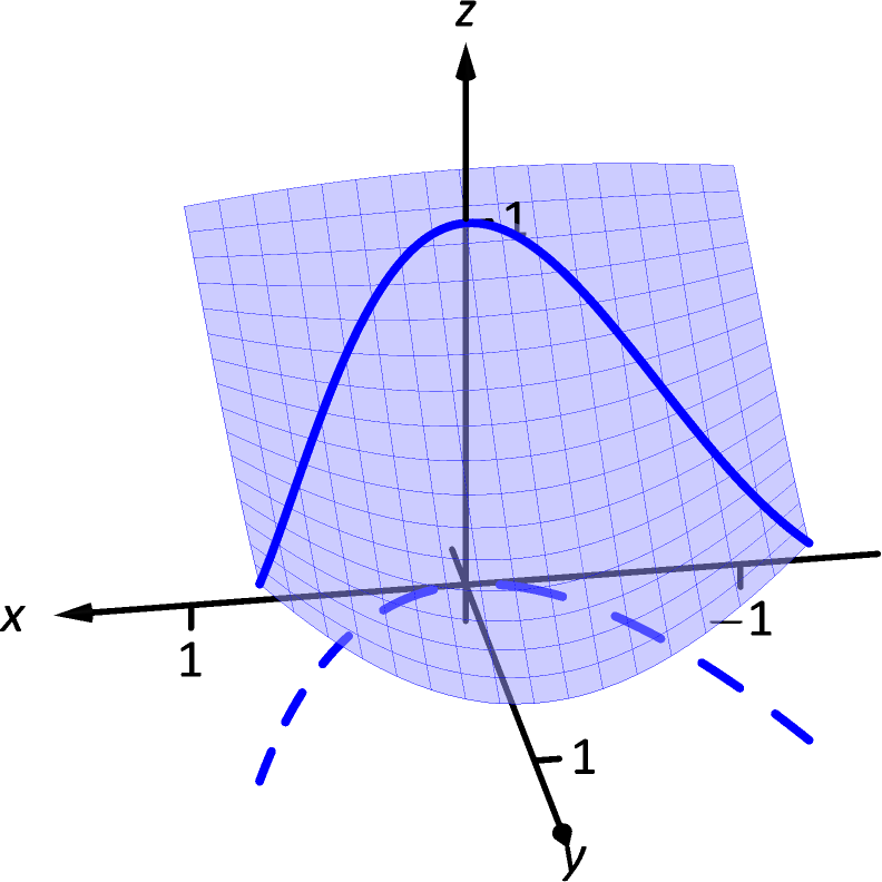 (a)
(a)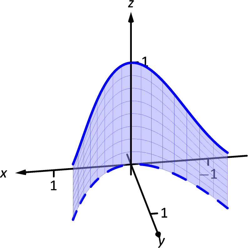 (b)
(b)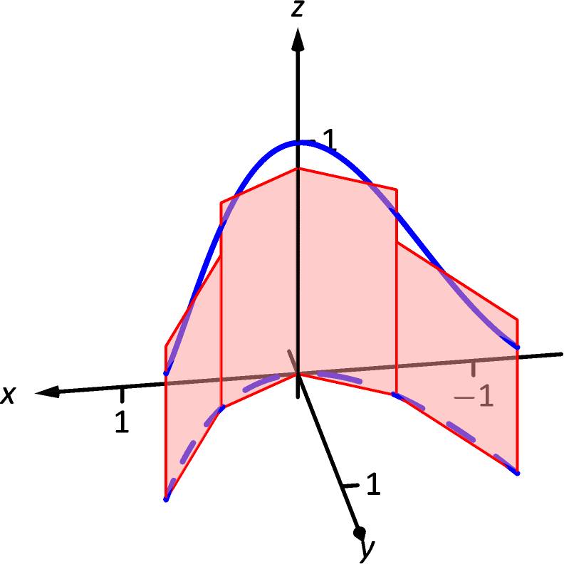 (c)
Figure 15.1.1: Finding area under a curve in space.
We first used integration to find “area under a curve.” In this section, we learn to do this (again), but in a different context.
Consider the surface and curve shown in Figure 15.1.1(a). The surface is given by . The dashed curve lies in the - plane and is the familiar parabola from ; we’ll call this curve . The curve drawn with a solid line in the graph is the curve in space that lies on our surface with and values that lie on .
The question we want to answer is this: what is the area that lies below the curve drawn with the solid line? In other words, what is the area of the region above and under the the surface ? This region is shown in Figure 15.1.1(b).
We suspect the answer can be found using an integral, but before trying to figure out what that integral is, let us first try to approximate its value.
In Figure 15.1.1(c), four rectangles have been drawn over the curve . The bottom corners of each rectangle lie on , and each rectangle has a height given by the function for some pair along between the rectangle’s bottom corners.
As we know how to find the area of each rectangle, we are able to approximate the area above and under . Clearly, our approximation will be an approximation. The heights of the rectangles do not match exactly with the surface , nor does the base of each rectangle follow perfectly the path of .
In typical calculus fashion, our approximation can be improved by using more rectangles. The sum of the areas of these rectangles gives an approximate value of the true area above and under . As the area of each rectangle is “height width”, we assert that the
When first learning of the integral, and approximating areas with “heights widths”, the width was a small change in : . That will not suffice in this context. Rather, each width of a rectangle is actually approximating the arc length of a small portion of . In Section 12.5, we used to represent the arc-length parameter of a curve. A small amount of arc length will thus be represented by .
The height of each rectangle will be determined in some way by the surface . If we parameterize by , an -value corresponds to an pair that lies on the parabola . Since is a function of and , and and are functions of , we can say that is a function of . Given a value , we can compute and find a height. Thus
| area under and above | ||||
| area under and above | ||||
| (15.1) |
Here we have introduce a new notation, the integral symbol with a subscript of . It is reminiscent of our usage of . Using the train of thought found in the Integration Review preceding this section, we interpret “” as meaning “sum up, along a curve , function values small arc lengths.” It is understood here that represents the arc-length parameter.
All this leads us to a definition. The integral found in Equation (15.1) is called a line integral. We formally define it below, but note that the definition is very abstract. On one hand, one is apt to say “the definition makes sense,” while on the other, one is equally apt to say “but I don’t know what I’m supposed to do with this definition.” We’ll address that after the definition, and actually find an answer to the area problem we posed at the beginning of this section.
Definition 15.1.1 Line Integral Over A Scalar Field
Let be a smooth curve parameterized by , the arc-length parameter, and let be a continuous function of . A line integral is an integral of the form
where is any partition of the -interval over which is defined, is any value in the subinterval, is the width of the subinterval, and is the length of the longest subinterval in the partition.
When is a closed curve, i.e., a curve that ends at the same point at which it starts, we use
The definition of the line integral does not specify whether is a curve in the plane or space (or hyperspace), as the definition holds regardless. For now, we’ll assume lies in the - plane.
This definition of the line integral doesn’t really say anything new. If is a curve and is the arc-length parameter of on , then
The real difference with this integral from the standard “” we used in the past is that of context. Our previous integrals naturally summed up values over an interval on the -axis, whereas now we are summing up values over a curve. If we can parameterize the curve with the arc-length parameter, we can evaluate the line integral just as before. Unfortunately, parameterizing a curve in terms of the arc-length parameter is usually very difficult, so we must develop a method of evaluating line integrals using a different parameterization.
Given a curve , find any smooth parameterization of : and , for continuous functions and , where . We can represent this parameterization with a vector-valued function, .
In Section 12.5, we defined the arc-length parameter in Equation (12.2) as
By the Fundamental Theorem of Calculus, . Because is smooth, this is strictly positive, and so has an inverse: . This means that and
We can now substitute to see that
We restate this as a theorem, along with its three-dimensional analogue, followed by an example where we finally evaluate an integral and find an area.
Theorem 15.1.1 Evaluating a Line Integral Over A Scalar Field
-
•
Let be a curve parameterized by , , where and are continuously differentiable, and let , where is continuous over . Then
-
•
Let be a curve parameterized by , , where , and are continuously differentiable, and let , where is continuous over . Then
To be clear, the first point of Theorem 15.1.1 can be used to find the area under a surface and above a curve . We will later give an understanding of the line integral when is a curve in space.
Let’s do an example where we actually compute an area.
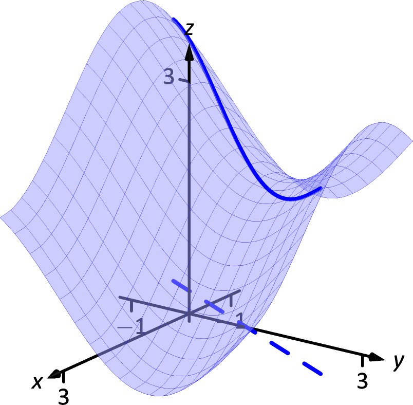 (a)
(a)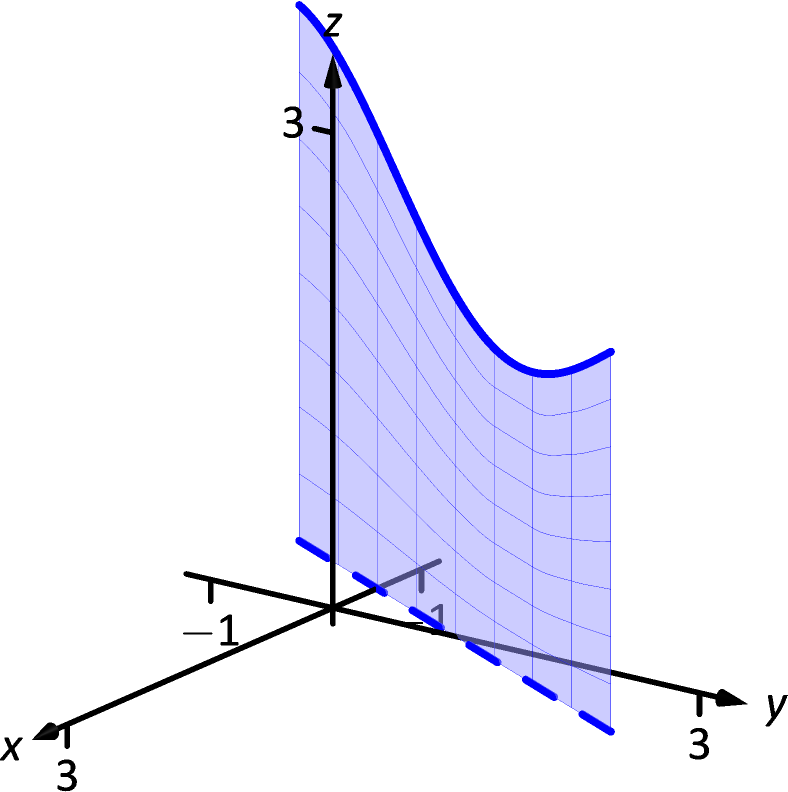 (b)
Figure 15.1.2: Finding area under a curve in Example 15.1.1.
Example 15.1.1 Evaluating a line integral: area under a surface over a curve.
Find the area under the surface over the curve , which is the segment of the line on , as shown in Figure 15.1.2.
SolutionOur first step is to represent with a vector-valued function. Since is a simple line, and we have a explicit relationship between and (namely, that is ), we can let , , and write for .
We find the values of over as . We also need ; with , we have . Thus .
The area we seek is
We will practice setting up and evaluating a line integral in another example, then find the area described at the beginning of this section.
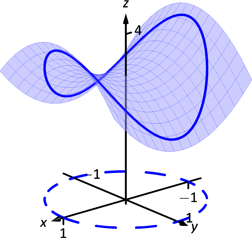 (a)
(a)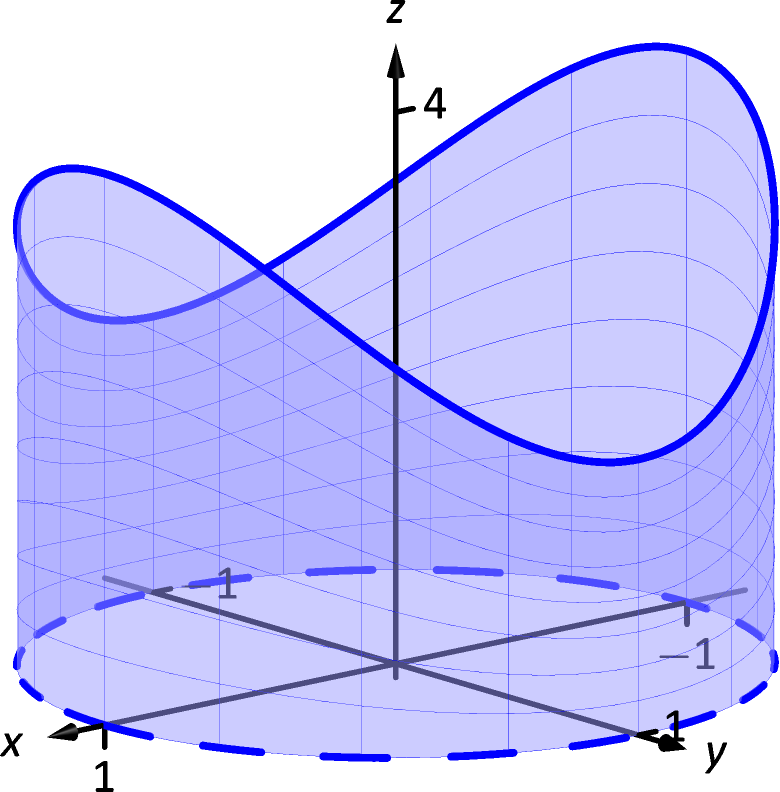 (b)
Figure 15.1.3: Finding area under a curve in Example 15.1.2.
Example 15.1.2 Evaluating a line integral: area under a surface over a curve.
Find the area over the unit circle in the - plane and under the surface , shown in Figure 15.1.3.
SolutionThe curve is the unit circle, which we will describe with the parameterization for . We find , so .
We find the values of over as . Thus the area we seek is (note the use of the notation):
(Note: we may have approximated this answer from the start. The unit circle has a circumference of , and we may have guessed that due to the apparent symmetry of our surface, the average height of the surface is 3.)
We now consider the example that introduced this section.
Example 15.1.3 Evaluating a line integral: area under a surface over a curve.
Find the area under and over the parabola , from .
SolutionWe parameterize our curve as for ; we find , so .
Replacing and with their respective functions of , we have . Thus the area under and over is found to be
| This integral is impossible to evaluate using the techniques developed in this text. We resort to a numerical approximation; accurate to two places after the decimal, we find the area is | ||||
We give one more example of finding area.
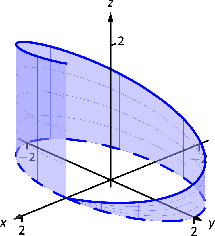 Figure 15.1.4: Finding area under a curve in Example 15.1.4.
Example 15.1.4 Evaluating a line integral: area under a curve in space.
Find the area above the - plane and below the helix parameterized by , for , as shown in Figure 15.1.4.
SolutionNote how this is problem is different than the previous examples: here, the height is not given by a surface, but by the curve itself.
We use the given vector-valued function to determine the curve in the - plane by simply using the first two components of : . Thus .
The height is not found by evaluating a surface over , but rather it is given directly by the third component of : . Thus
where the approximation was obtained using numerical methods.
Note how in each of the previous examples we are effectively finding “area under a curve”, just as we did when first learning of integration. We have used the phrase “area over a curve and under a surface,” but that is because of the important role plays in the integral. The figures show how the curve defines another curve on the surface , and we are finding the area under that curve.
Properties of Line Integrals
Many properties of line integrals can be inferred from general integration properties. For instance, if is a scalar, then .
One property in particular of line integrals is worth noting. If is a curve composed of subcurves and , where they share only one point in common (see Figure 15.1.5(a)), then the line integral over is the sum of the line integrals over and :
This property allows us to evaluate line integrals over some curves that are not smooth. Note how in Figure 15.1.5(b) the curve is not smooth at , so by our definition of the line integral we cannot evaluate . However, one can evaluate line integrals over and and their sum will be the desired quantity.
A curve that is composed of two or more smooth curves is said to be piecewise smooth. In this chapter, any statement that is made about smooth curves also holds for piecewise smooth curves.
We state these properties as a theorem.
Theorem 15.1.2 Properties of Line Integrals Over Scalar Fields
-
1.
Let be a smooth curve parameterized by the arc-length parameter , let and be continuous functions of , and let and be scalars. Then
-
2.
Let be piecewise smooth, composed of smooth components and . Then
Mass and Center of Mass
We first learned integration as a method to find area under a curve, then later used integration to compute a variety of other quantities, such as arc length, volume, force, etc. In this section, we also introduced line integrals as a method to find area under a curve, and now we explore one more application.
Let a curve (either in the plane or in space) represent a thin wire with variable density . We can approximate the mass of the wire by dividing the wire (i.e., the curve) into small segments of length and assume the density is constant across these small segments. The mass of each segment is density of the segment its length; by summing up the approximate mass of each segment we can approximate the total mass:
By taking the limit as the length of the segments approaches 0, we have the definition of the line integral as seen in Definition 15.1.1. When learning of the line integral, we let represent a height; now we let represent a density.
We can extend this understanding of computing mass to also compute the center of mass of a thin wire. (As a reminder, the center of mass can be a useful piece of information as objects rotate about that center.) We give the relevant formulas in the next definition, followed by an example. Note the similarities between this definition and Definition 14.6.4, which gives similar properties of solids in space.
Definition 15.1.2 Mass, Center of Mass of Thin Wire
Let a thin wire lie along a smooth curve with continuous density function , where is the arc length parameter.
-
1.
The mass of the thin wire is .
-
2.
The moment about the - plane is .
-
3.
The moment about the - plane is .
-
4.
The moment about the - plane is .
-
5.
The center of mass of the wire is
Example 15.1.5 Evaluating a line integral: calculating mass.
A thin wire follows the path , . The density of the wire is determined by its position in space: gm/cm. The wire is shown in Figure 15.1.6, where a light color indicates low density and a dark color represents high density. Find the mass and center of mass of the wire.††margin:
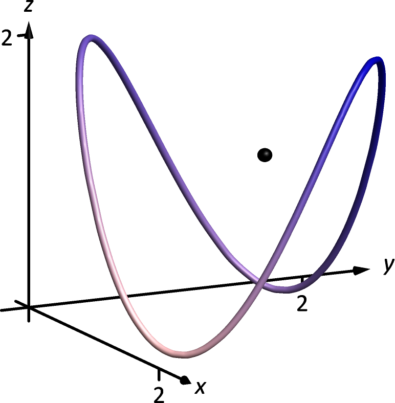 Figure 15.1.6: Finding the mass of a thin wire in Example 15.1.5.
SolutionWe compute the density of the wire as
We compute as
Thus the mass is
We compute the moments about the coordinate planes:
Thus the center of mass of the wire is located at
as indicated by the dot in Figure 15.1.6. Note how in this example, the curve is “centered” about the point , though the variable density of the wire pulls the center of mass out along the and axes.
We end this section with a callback to the Integration Review that preceded this section. A line integral looks like: . As stated before the definition of the line integral, this means “sum up, along a curve , function values small arc lengths.” When represents a height, we have “height length = area.” When is a density (and we use by convention), we have “density (mass per unit length) length = mass.”
In the next section, we investigate a new mathematical object, the vector field. The remaining sections of this chapter are devoted to understanding integration in the context of vector fields.
Exercises 15.1
Terms and Concepts
-
1.
Explain how a line integral can be used to find the area under a curve.
-
2.
How does the evaluation of a line integral given as differ from a line integral given as ?
-
3.
Why are most line integrals evaluated using Theorem 15.1.1 instead of “directly” as ?
-
4.
Sketch a closed, piecewise smooth curve composed of three subcurves.
Problems
In Exercises 5–18, a planar curve is given along with a surface that is defined over . Evaluate the line integral
-
5.
is the line segment joining the points and ; the surface is .
-
6.
is the segment of on ; the surface is .
-
7.
is the circle with radius 2 centered at the point ; the surface is .
-
8.
is the curve given by on ; the surface is .
-
9.
is the piecewise curve composed of the line segments that connect to , then connect to ; the surface is .
-
10.
is the piecewise curve composed of the line segment joining the points and , along with the quarter-circle parametrized by on (which starts at the point and ends at ; the surface is .
-
11.
is the arc of the unit circle traced from to ; the surface is .
-
12.
is the line segment from to ; the surface is
-
13.
is polygonal path from to to ; the surface is
-
14.
is the path from counterclockwise along the circle to the point and then back to along the -axis; the surface is
-
15.
is the curve for ; the surface is .
-
16.
is the helix , , for ; the surface is
-
17.
is the curve , , for ; the surface is
-
18.
is the curve , , for ; the surface is
In Exercises 19–22, a planar curve is given along with a surface that is defined over . Set up the line integral , then approximate its value using technology.
-
19.
is the portion of the parabola on ; the surface is .
-
20.
is the portion of the curve on ; the surface is .
-
21.
is the ellipse given by on ; the surface is .
-
22.
is the portion of on ; the surface is .
In Exercises 23–26, a parametrized curve in space is given. Find the area above the - plane that is under .
-
23.
: for .
-
24.
: for .
-
25.
: for .
-
26.
: for .
In Exercises 27–28, a parametrized curve is given that represents a thin wire with density . Find the mass and center of mass of the thin wire.
-
27.
: for ; g/cm.
-
28.
: for ; g/cm. Use technology to approximate the value of each integral.
-
29.
Use a line integral to find the lateral surface area of the part of the cylinder below the plane and above the -plane.
-
30.
Prove that the Riemann integral is a special case of a line integral.
-
31.
Let be a curve whose arc length is . Show that .
